Classifying system models and simulation with MATLAB

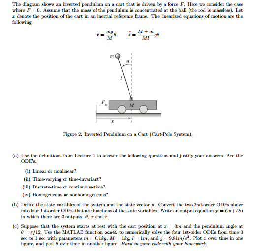
The diagram shows an inverted pendulum on a cart that is driven by a force F. Here we consider the case where F = 0. Assume that the mass of the pendulum is concentrated at the ball (the rod is massless). Let x denote the position of the cart in an inertial reference frame. The linearized equations of motion are the following: x^- = mg/M theta, theta^- = M+m/Ml g theta Use the definitions from Lecture 1 to answer the following questions and justify your answers. Are the ODE's: Use the definitions from Lecture 1 to answer the following questions and justify your answers. Are the ODEs: Linear or nonlinear? Time-varying or time-invariant? Discrete-time or continuous-time? Homogeneous or nonhomogeneous? Define the state variables of the system and the state vector x. Convert the two 2nd-order ODEs above into four 1st-order ODEs that are functions of the state variables. Write an output equation y = Cx+Du in which there are 3 outputs, theta, x and x^.. Suppose that the system starts at rest with the cart position at x = 0m and the pendulum angle at theta = pi/12. Use the MATLAB function ode45 to numerically solve the four 1st-order ODEs from time 0 sec to 1 sec with parameters m = 0.1 kg, M = 1kg, l = 1m, and g = 9.81m/s^2. Plot x over time in one figure, and plot theta over time in another figure. Hand in your code th your