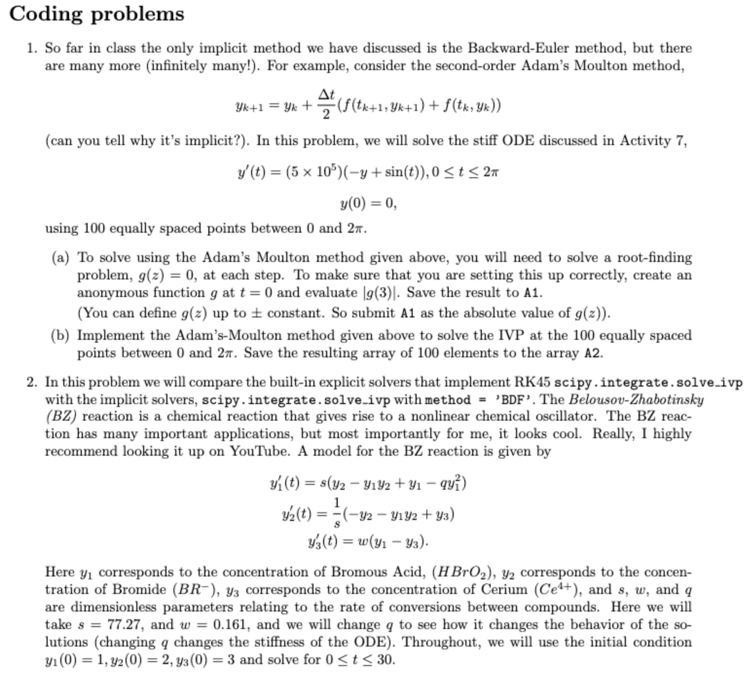
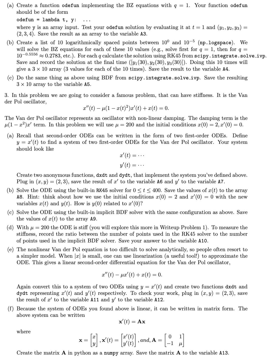
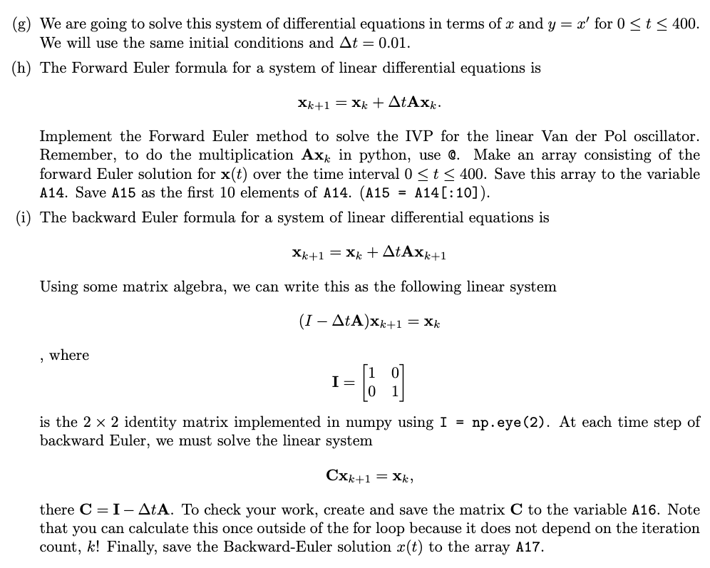
Coding problems 1. So far in class the only implicit method we have discussed is the Backward-Euler method, but there are many more (infinitely many!). For example, consider the second-order Adam's Moulton method, At Yk+1 = Yk+(f(tk+1, Yk+1) + f(tk, yk)) 2 (can you tell why it's implicit?). In this problem, we will solve the stiff ODE discussed in Activity 7, y' (t) = (5 x 105)(-y+sin(t)), 0 t 2 y(0) = 0, using 100 equally spaced points between 0 and 2. (a) To solve using the Adam's Moulton method given above, you will need to solve a root-finding problem, g(z) = 0, at each step. To make sure that you are setting this up correctly, create an anonymous function g at t = 0 and evaluate [g(3)|. Save the result to A1. (You can define g(z) up to constant. So submit A1 as the absolute value of g(z)). (b) Implement the Adam's-Moulton method given above to solve the IVP at the 100 equally spaced points between 0 and 27. Save the resulting array of 100 elements to the array A2. 2. In this problem we will compare the built-in explicit solvers that implement RK45 scipy. integrate.solve_ivp with the implicit solvers, scipy. integrate.solve_ivp with method = 'BDF'. The Belousov-Zhabotinsky (BZ) reaction is a chemical reaction that gives rise to a nonlinear chemical oscillator. The BZ reac- tion has many important applications, but most importantly for me, it looks cool. Really, I highly recommend looking it up on YouTube. A model for the BZ reaction is given by y (t) = s(y2 - Y1Y2 + 9 qy) y(t) = ( 8 (-Y2 - Y1y2 + Y3) y(t) = w(y Y3). - Here y corresponds to the concentration of Bromous Acid, (HBrO), 32 corresponds to the concen- tration of Bromide (BR), y3 corresponds to the concentration of Cerium (Ce+), and s, w, and q are dimensionless parameters relating to the rate of conversions between compounds. Here we will take s = 77.27, and w = 0.161, and we will change q to see how it changes the behavior of the so- lutions (changing q changes the stiffness of the ODE). Throughout, we will use the initial condition y (0) = 1, y2 (0) = 2, y3 (0) = 3 and solve for 0 < t < 30. (a) Create a function odefun implementing the BZ equations with q = 1. Your function odefun should be of the form odefun lambda t, y: where y is an array input. Test your odefun solution by evaluating it at t = 1 and (y, 92, Y3) (2, 3, 4). Save the result as an array to the variable A3. (b) Create a list of 10 logarithmically spaced points between 100 and 10-5 (np.logspace). We will solve the BZ equations for each of these 10 values (e.g., solve first for q = 1, then for q = 10-0.5556 0.2783, etc.). For each q calculate the solution using RK45 from scipy. integrate. solve_ivp. Save and record the solution at the final time ([y (30), y2 (30), y3 (30)]). Doing this 10 times will give a 3 10 array (3 values for each of the 10 times). Save the result to the variable A4. (c) Do the same thing as above using BDF from scipy.integrate.solve_ivp. Save the resulting 3 x 10 array to the variable A5. 3. In this problem we are going to consider a famous problem, that can have stiffness. It is the Van der Pol oscillator, x"(t) - (1 x(t))x' (t) + x(t) = 0. The Van der Pol oscillator represents an oscillator with non-linear damping. The damping term is the (1-x)x' term. In this problem we will use = 200 and the initial conditions x(0) = 2, x' (0) = 0. (a) Recall that second-order ODEs can be written in the form of two first-order ODEs. Define y = x'(t) to find a system of two first-order ODEs for the Van der Pol oscillator. Your system should look like x' (t) y' (t) Create two anonymous functions, dxdt and dydt, that implement the system you've defined above. Plug in (x, y) = (2, 3), save the result of x' to the variable A6 and y' to the variable A7. (b) Solve the ODE using the built-in RK45 solver for 0 t 400. Save the values of x(t) to the array A8. Hint: think about how we use the initial conditions (0) = 2 and x'(0) =0 with the new variables x(t) and y(t). How is y(0) related to x'(0)? (c) Solve the ODE using the built-in implicit BDF solver with the same configuration as above. Save the values of x(t) to the array A9. (d) With = 200 the ODE is stiff (you will explore this more in Writeup Problem 1). To measure the stiffness, record the ratio between the number of points used in the RK45 solver to the number of points used in the implicit BDF solver. Save your answer to the variable A10. (e) The nonlinear Van der Pol equation is too difficult to solve analytically, so people often resort to a simpler model. When || is small, one can use linearization (a useful tool!) to approximate the ODE. This gives a linear second-order differential equation for the Van der Pol oscillator, x" (t) x' (t) + x(t) = where Again convert this to a system of two ODEs using y = x' (t) and create two functions dxdt and dydt representing x'(t) and y'(t) respectively. To check your work, plug in (x, y) = (2,3), save the result of x' to the variable A11 and y' to the variable A12. (f) Because the system of ODEs you found above is linear, it can be written in matrix form. The above system can be written = 0. x' (t): = Ax X = - [*] x (t) = [~ (8)], and, A = [ , x' Create the matrix A in python as a numpy array. Save the matrix A to the variable A13. (g) We are going to solve this system of differential equations in terms of x and y = x' for 0 t 400. We will use the same initial conditions and At = 0.01. (h) The Forward Euler formula for a system of linear differential equations is Xk+1=Xk + AtAxk. Implement the Forward Euler method to solve the IVP for the linear Van der Pol oscillator. Remember, to do the multiplication Ax in python, use @. Make an array consisting of the forward Euler solution for x(t) over the time interval 0 t 400. Save this array to the variable A14. Save A15 as the first 10 elements of A14. (A15 A14 [:10]). = (i) The backward Euler formula for a system of linear differential equations is Xk+1=Xk+AtAXk+1 Using some matrix algebra, we can write this as the following linear system (I AtA)Xk+1=Xk " where -69 I= is the 2 2 identity matrix implemented in numpy using I = np.eye (2). At each time step of backward Euler, we must solve the linear system CXk+1= Xk, there CI- AtA. To check your work, create and save the matrix C to the variable A16. Note that you can calculate this once outside of the for loop because it does not depend on the iteration count, k! Finally, save the Backward-Euler solution r(t) to the array A17.