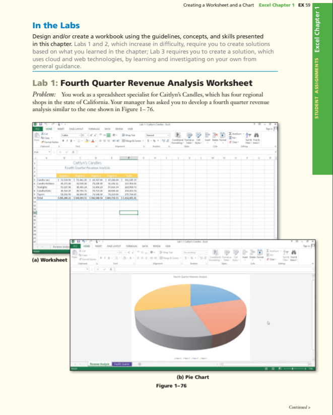
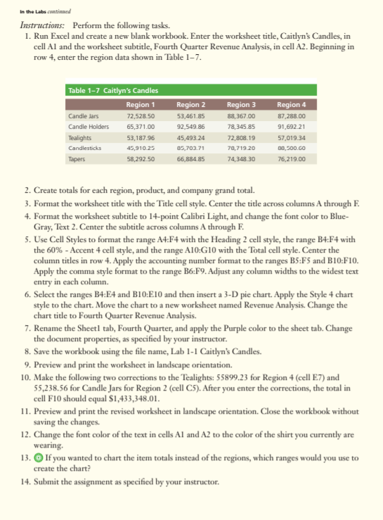
Creating a Worksheet and a Chart Excel Chapter 1 EX 59 In the Labs Design and/or create a workbook using the guidelines, concepts, and skills presented in this chapter. Labs 1 and 2, which increase in difficulty, require you to create solutions based on what you learned in the chapter; Lab 3 requires you to create a solution, which uses cloud and web technologies, by learning and investigating on your own from general guidance. Lab 1: Fourth Quarter Revenue Analysis Worksheet Problem: You work as a spreadsheet specialist for Caitlyn's Candles, which has four regional shops in the state of California. Your manager has asked you to develop a fourth quarter revenue analysis similar to the one shown in Figure 1-76. STUDENT ASSIGNMENTS Excel Chapter 1 2 Caitlyn's Candles Fouth Carter FAH a 52. SS15 SLALO4 (a) Worksheet (b) Pie Chart Figure 1-76 Contd> In the Labs continued Instructions: Perform the following tasks. 1. Run Excel and create a new blank workbook. Enter the worksheet title, Caitlyn's Candles, in cell Al and the worksheet subtitle, Fourth Quarter Revenue Analysis, in cell A2. Beginning in row 4, enter the region data shown in Table 1-7. Table 1-7 Caitlyn's Candles Region 1 Candle dars 72,528.50 Candle Holders 65,371.00 Tealights 53,187.96 Candlesticks 45,910.25 Tapers 58,292.50 Region 2 53,461.85 92,549.86 45,493.24 85,703.71 66,884.85 Region 3 88,367.00 78,345.85 72,808.19 78,719.20 74,348.30 Region 4 87,288.00 91,692.21 57,019.34 38,500.GO 76,219.00 2. Create totals for each region, product, and company grand total. 3. Format the worksheet title with the Title cell style. Center the title across columns A through F. 4. Format the worksheet subtitle to 14-point Calibri Light, and change the font color to Blue- Gray, Text 2. Center the subtitle across columns A through F. 5. Use Cell Styles to format the range A4:F4 with the Heading 2 cell style, the range B4:54 with the 60% - Accent 4 cell style, and the range A10:10 with the Total cell style. Center the column titles in row 4. Apply the accounting number format to the ranges B5:F5 and B10:F10. Apply the comma style format to the range B6:F9. Adjust any column widths to the widest text entry in each column. 6. Select the ranges B4:E4 and B10:E10 and then insert a 3-D pie chart. Apply the Style 4 chart style to the chart. Move the chart to a new worksheet named Revenue Analysis. Change the chart title to Fourth Quarter Revenue Analysis. 7. Rename the Sheetl tab, Fourth Quarter, and apply the Purple color to the sheet tab. Change the document properties, as specified by your instructor. 8. Save the workbook using the file name, Lab 1-1 Caitlyn's Candles. 9. Preview and print the worksheet in landscape orientation 10. Make the following two corrections to the Tealights: 55899.23 for Region 4 (cell E7) and 55,238.56 for Candle Jars for Region 2 (cell C5). After you enter the corrections, the total in cell F10 should equal $1,433,348.01. 11. Preview and print the revised worksheet in landscape orientation. Close the workbook without saving the changes. 12. Change the font color of the text in cells Al and A2 to the color of the shirt you currently are wearing 13. If you wanted to chart the item totals instead of the regions, which ranges would you use to create the chart? 14. Submit the assignment as specified by your instructor