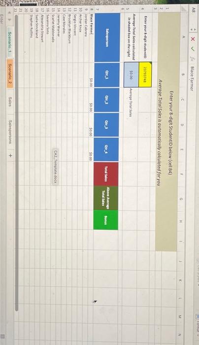
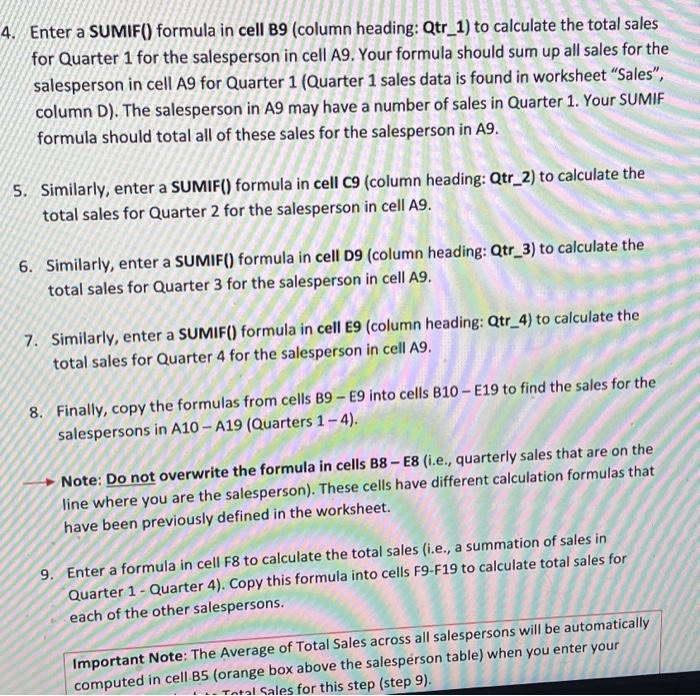
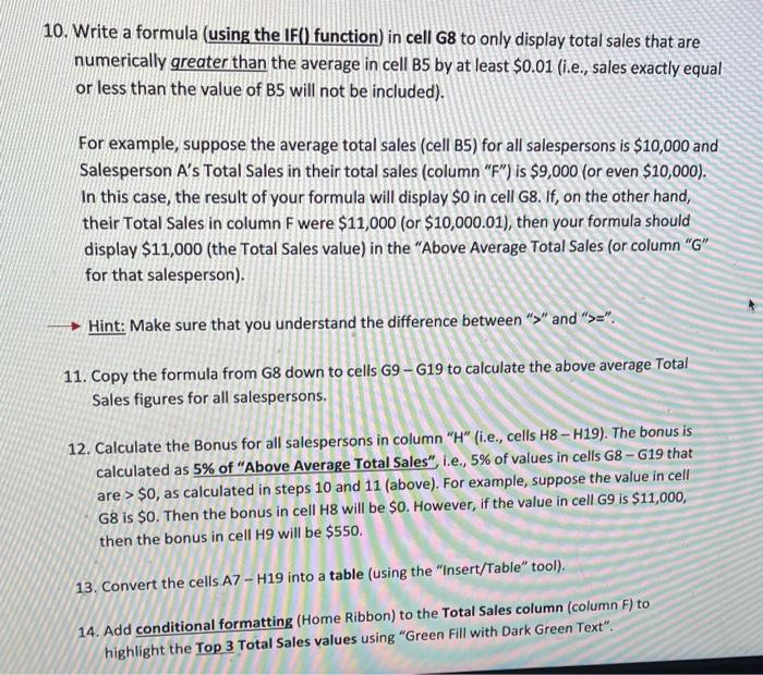
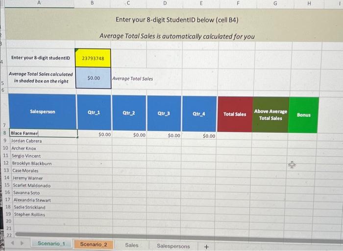
Enter a SUMIF() formula in cell B9 (column heading: Qtr_1) to calculate the total sales for Quarter 1 for the salesperson in cell A9. Your formula should sum up all sales for the salesperson in cell A9 for Quarter 1 (Quarter 1 sales data is found in worksheet "Sales", column D). The salesperson in A9 may have a number of sales in Quarter 1. Your SUMIF formula should total all of these sales for the salesperson in A9. 5. Similarly, enter a SUMIF() formula in cell C9 (column heading: Qtr_2) to calculate the total sales for Quarter 2 for the salesperson in cell A9. 6. Similarly, enter a SUMIF() formula in cell D9 (column heading: Qtr_3) to calculate the total sales for Quarter 3 for the salesperson in cell A9. 7. Similarly, enter a SUMIF() formula in cell E9 (column heading: Qtr_4) to calculate the total sales for Quarter 4 for the salesperson in cell A9. 8. Finally, copy the formulas from cells B9 - E9 into cells B10 - E19 to find the sales for the salespersons in A10 - A19 (Quarters 14). Note: Do not overwrite the formula in cells B8 - E8 (i.e., quarterly sales that are on the line where you are the salesperson). These cells have different calculation formulas that have been previously defined in the worksheet. 9. Enter a formula in cell F8 to calculate the total sales (i.e., a summation of sales in Quarter 1 - Quarter 4). Copy this formula into cells F9-F19 to calculate total sales for each of the other salespersons. Important Note: The Average of Total Sales across all salespersons will be automatically computed in cell B5 (orange box above the salesperson table) when you enter your 10. Write a formula (using the IF() function) in cell G8 to only display total sales that are numerically greater than the average in cell B5 by at least $0.01 (i.e., sales exactly equal or less than the value of B5 will not be included). For example, suppose the average total sales (cell B5) for all salespersons is $10,000 and Salesperson A's Total Sales in their total sales (column "F") is $9,000 (or even $10,000 ). In this case, the result of your formula will display $0 in cell G8. If, on the other hand, their Total Sales in column F were $11,000 (or $10,000.01 ), then your formula should display $11,000 (the Total Sales value) in the "Above Average Total Sales (or column " G " for that salesperson). Hint: Make sure that you understand the difference between " > " and " >==. 11. Copy the formula from G8 down to cells G9G19 to calculate the above average Total Sales figures for all salespersons. 12. Calculate the Bonus for all salespersons in column " H " (i.e., cells H8H19). The bonus is calculated as 5% of "Above Average Total Sales", i.e., 5\% of values in cells G8 - G19 that are >$0, as calculated in steps 10 and 11 (above). For example, suppose the value in cell G8 is $0. Then the bonus in cell H8 will be $0. However, if the value in cell G9 is $11,000, then the bonus in cell H9 will be $550. 13. Convert the cells A7 - H19 into a table (using the "Insert/Table" tool). 14. Add conditional formatting (Home Ribbon) to the Total Sales column (column F) to highlight the Top 3 Total Sales values using "Green Fill with Dark Green Text