Fill in the column with the correct formulas.

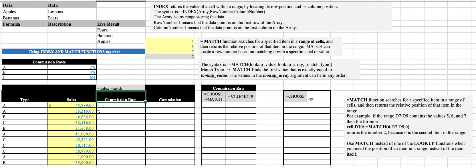
Data Apples Bananas Formula Data Lemons Pears Description INDEX returns the value of a cell within a range, by locating its row position and its column position. The syntax is: =INDEX(Array,RowNumber,ColumnNumber) The Array is any range storing the data. RowNumber 1 means that the data point is on the first row of the Array. ColumnNumber 1 means that the data point is on the first column on the Array. Live Result Pears Bananas Apples 5 6 7 2 = MATCH function searches for a specified item in a range of cells, and then returns the relative position of that item in the range. MATCH can locate a row number based on matching it with a specific label or value. Using INDEX AND MATCH FUNCTIONS together Commission Rates A B Ic 2% 4% 6% The syntax is: =MATCH(lookup_value, lookup_array, [match_type]) Match Type O- MATCH finds the first value that is exactly equal to lookup_value. The values in the lookup_array argument can be in any order. =index==match Commission Rate =CHOOSE =MATCH VL00KUP =CHOOSE Type Commission Rate Commission =IF A A B B A A B Sales 45,789.00 = 35.216.00 4,636.00 32,516.00 21,658.00 11,000.00 45,321.00 70,111.00 58,999.00 1,000.00 35,000.00 =MATCH function searches for a specified item in a range of cells, and then returns the relative position of that item in the range. For example, if the range D7:D9 contains the values 5, 6, and 7, then the formula cell D10:=MATCH(6,D7:D9,0) returns the number 2, because 6 is the second item in the range. Use MATCH instead of one of the LOOKUP functions when you need the position of an item in a range instead of the item itself. Data Apples Bananas Formula Data Lemons Pears Description INDEX returns the value of a cell within a range, by locating its row position and its column position. The syntax is: =INDEX(Array,RowNumber,ColumnNumber) The Array is any range storing the data. RowNumber 1 means that the data point is on the first row of the Array. ColumnNumber 1 means that the data point is on the first column on the Array. Live Result Pears Bananas Apples 5 6 7 2 = MATCH function searches for a specified item in a range of cells, and then returns the relative position of that item in the range. MATCH can locate a row number based on matching it with a specific label or value. Using INDEX AND MATCH FUNCTIONS together Commission Rates A B Ic 2% 4% 6% The syntax is: =MATCH(lookup_value, lookup_array, [match_type]) Match Type O- MATCH finds the first value that is exactly equal to lookup_value. The values in the lookup_array argument can be in any order. =index==match Commission Rate =CHOOSE =MATCH VL00KUP =CHOOSE Type Commission Rate Commission =IF A A B B A A B Sales 45,789.00 = 35.216.00 4,636.00 32,516.00 21,658.00 11,000.00 45,321.00 70,111.00 58,999.00 1,000.00 35,000.00 =MATCH function searches for a specified item in a range of cells, and then returns the relative position of that item in the range. For example, if the range D7:D9 contains the values 5, 6, and 7, then the formula cell D10:=MATCH(6,D7:D9,0) returns the number 2, because 6 is the second item in the range. Use MATCH instead of one of the LOOKUP functions when you need the position of an item in a range instead of the item itself