For Problems 2022, download the spreadsheet containing the data used to prepare Table 5.3,

Rates of return, 19262013, from Connect.

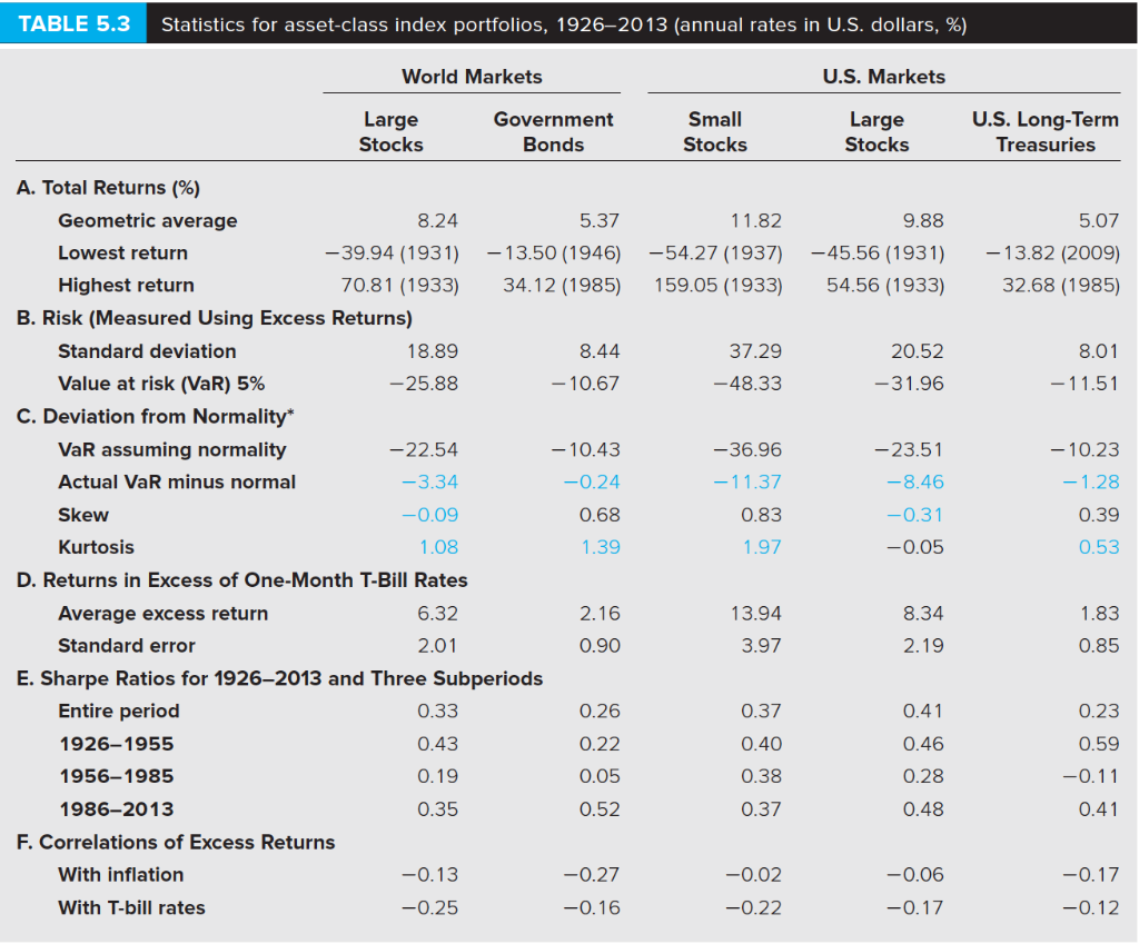
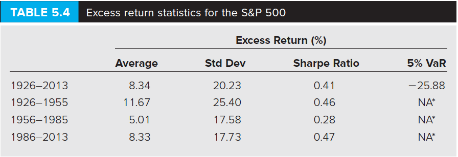
20. Calculate the same subperiod means and standard deviations for small stocks as

Table 5.4 of the text provides for large stocks. (LO 5-2)

a. Have small stocks provided better reward-to-volatility (Sharpe) ratios than large stocks?

b. Do small stocks show a similar higher standard deviation in the earliest subperiod as

Table 5.4 documents for large stocks?

I know the instructions say to download the data used to prepare table 5.3. However, my professor did not give me access to the connect software, so I was wondering if the above questions could answered despite not having that info?

Thank you!

TABLE 5.3 Statistics for asset-class index portfolios, 19262013 (annual rates in U.S. dollars, %) World Markets U.S. Markets Large Government Bonds Small Stocks Large Stocks U.S. Long-Term Treasuries Stocks 11.82 -54.27 (1937) 159.05 (1933) 9.88 -45.56 (1931) 54.56 (1933) 5.07 13.82 (2009) 32.68 (1985) 8.01 37.29 -48.33 20.52 -31.96 11.51 A. Total Returns (%) Geometric average 8.24 5.37 Lowest return - 39.94 (1931) 13.50 (1946) Highest return 70.81 (1933) 34.12 (1985) B. Risk (Measured Using Excess Returns) Standard deviation 18.89 8.44 Value at risk (VaR) 5% -25.88 - 10.67 C. Deviation from Normality* VaR assuming normality -22.54 -10.43 Actual VaR minus normal -3.34 -0.24 Skew -0.09 0.68 Kurtosis 1.08 1.39 D. Returns in Excess of One-Month T-Bill Rates Average excess return 6.32 2.16 Standard error 2.01 0.90 E. Sharpe Ratios for 19262013 and Three Subperiods Entire period 0.33 0.26 1926-1955 0.43 0.22 1956-1985 0.19 0.05 1986-2013 0.35 0.52 F. Correlations of Excess Returns With inflation -0.13 -0.27 With T-bill rates -0.25 -0.16 -36.96 -11.37 0.83 1.97 -23.51 -8.46 -0.31 -0.05 - 10.23 1.28 0.39 0.53 1.83 13.94 3.97 8.34 2.19 0.85 0.37 0.40 0.38 0.37 0.41 0.46 0.28 0.48 0.23 0.59 -0.11 0.41 -0.02 -0.22 -0.06 -0.17 -0.17 -0.12 TABLE 5.4 Excess return statistics for the S&P 500, Excess Return (%) Average Std Dev Sharpe Ratio 5% VaR -25.88 NA* 19262013 19261955 19561985 1986-2013 8.34 11.67 5.01 8.33 20.23 25.40 17.58 17.73 0.41 0.46 0.28 0.47 NA* NA* TABLE 5.3 Statistics for asset-class index portfolios, 19262013 (annual rates in U.S. dollars, %) World Markets U.S. Markets Large Government Bonds Small Stocks Large Stocks U.S. Long-Term Treasuries Stocks 11.82 -54.27 (1937) 159.05 (1933) 9.88 -45.56 (1931) 54.56 (1933) 5.07 13.82 (2009) 32.68 (1985) 8.01 37.29 -48.33 20.52 -31.96 11.51 A. Total Returns (%) Geometric average 8.24 5.37 Lowest return - 39.94 (1931) 13.50 (1946) Highest return 70.81 (1933) 34.12 (1985) B. Risk (Measured Using Excess Returns) Standard deviation 18.89 8.44 Value at risk (VaR) 5% -25.88 - 10.67 C. Deviation from Normality* VaR assuming normality -22.54 -10.43 Actual VaR minus normal -3.34 -0.24 Skew -0.09 0.68 Kurtosis 1.08 1.39 D. Returns in Excess of One-Month T-Bill Rates Average excess return 6.32 2.16 Standard error 2.01 0.90 E. Sharpe Ratios for 19262013 and Three Subperiods Entire period 0.33 0.26 1926-1955 0.43 0.22 1956-1985 0.19 0.05 1986-2013 0.35 0.52 F. Correlations of Excess Returns With inflation -0.13 -0.27 With T-bill rates -0.25 -0.16 -36.96 -11.37 0.83 1.97 -23.51 -8.46 -0.31 -0.05 - 10.23 1.28 0.39 0.53 1.83 13.94 3.97 8.34 2.19 0.85 0.37 0.40 0.38 0.37 0.41 0.46 0.28 0.48 0.23 0.59 -0.11 0.41 -0.02 -0.22 -0.06 -0.17 -0.17 -0.12 TABLE 5.4 Excess return statistics for the S&P 500, Excess Return (%) Average Std Dev Sharpe Ratio 5% VaR -25.88 NA* 19262013 19261955 19561985 1986-2013 8.34 11.67 5.01 8.33 20.23 25.40 17.58 17.73 0.41 0.46 0.28 0.47 NA* NA*