Gradient Descent Optimization

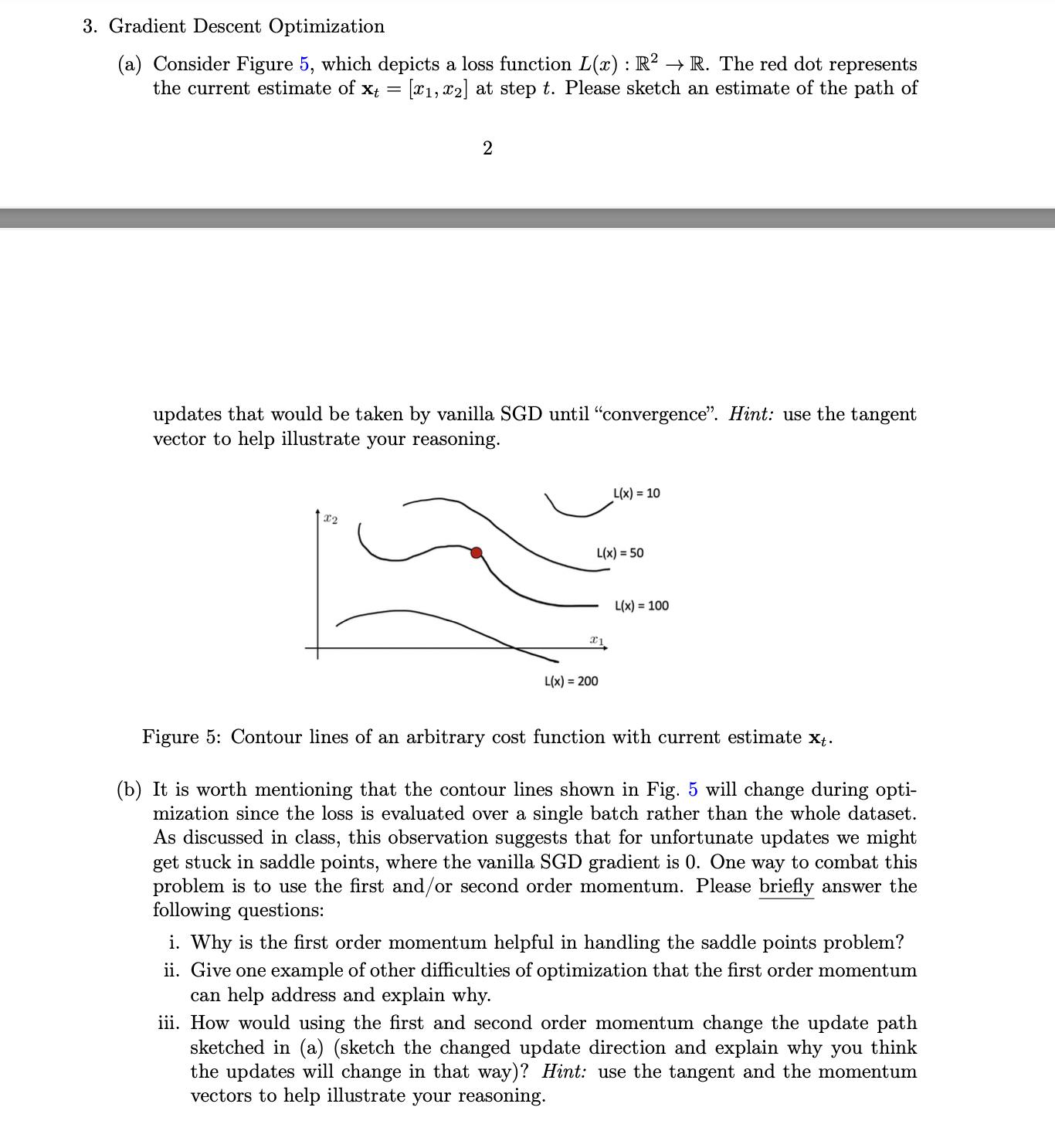
$($a$)$ Consider Figure $5,$ which depicts a loss function L$($x$)$:R$^(2)$rarrR$.$ The red dot represents the current estimate of x$\_($t$)=[$x$\_(1),$x$\_(2)]$ at step t$.$ Please sketch an estimate of the path of updates that would be taken by vanilla SGD until "convergence". Hint: use the tangent vector to help illustrate your reasoning. Figure $5$: Contour lines of an arbitrary cost function with current estimate x$\_($t$).$

$($b$)$ It is worth mentioning that the contour lines shown in Fig. $5$ will change during optimization since the loss is evaluated over a single batch rather than the whole dataset. As discussed in class, this observation suggests that for unfortunate updates we might get stuck in saddle points, where the vanilla SGD gradient is $0.$ One way to combat this problem is to use the first and$/$or second order momentum. Please briefly answer the following questions:

i$.$ Why is the first order momentum helpful in handling the saddle points problem?

ii$.$ Give one example of other difficulties of optimization that the first order momentum

can help address and explain why.

iii. How would using the first and second order momentum change the update path sketched in $($a$)($sketch the changed update direction and explain why you think the updates will change in that way$)?$ Hint: use the tangent and the momentum vectors to help illustrate your reasoning.