How to use lookup formulas at step9

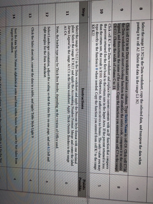
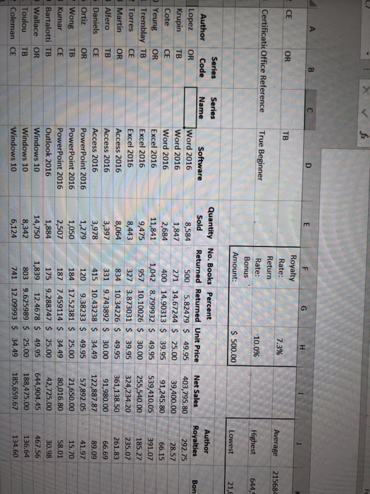
Select the range LI N2in the Data worksheet,copy the selected data, and transpose the data when pasting it to cell A2. Delete the data in the range L1:N2 8 4 ek cell C6 in the Data worksheet and inserta column Type Series Natme in dell C6 the Data worksheet and insert a lookup function that identifies the series code, compares it to the series legend, and then returns the name of the series. Copy the function you entered 8 e width of column C to 18 cell K7 in the Data worksheet and replace the current contents with an IF function that compares the percent returned for the first book to the return rate in the Input Area. If the percent returned is less 10 than the return rate, the result is $500. Otherwise, the author receives no bonus. The only value you may type directly in the function is 0 where needed. Copy the function you entered from cell K7 to the range K8:K22 Points Instructions Select the range G7:G22 in the Data worksheet and apply the Percent Style format with one decimal place. Select the range K7 K22 and apply the Accounting Number Format. Merge and center the label Series Legend in the range A1:C1 in the Data worksheet. Apply Thick Outside Borders to the range A1:C4 Note, the border type may be Thick Box Border, depending on the version of Office used 12 Seledt Select Landscape orientation, adjust the scaling so that the data fits on one page, and set 0.1 left and right margins for the Data worksheet Click the Sales sheet tab, convert the data to a table, and apply Table Style Light 9. 3 Sort the data by Series Name in alphabetical order and then within Series Name, sort by Net Sales from largest to smallest. 14