

Question: Insert a funnel chart of the data in the range F 8 :G 1 3 . Move and resize the chart to cover the range
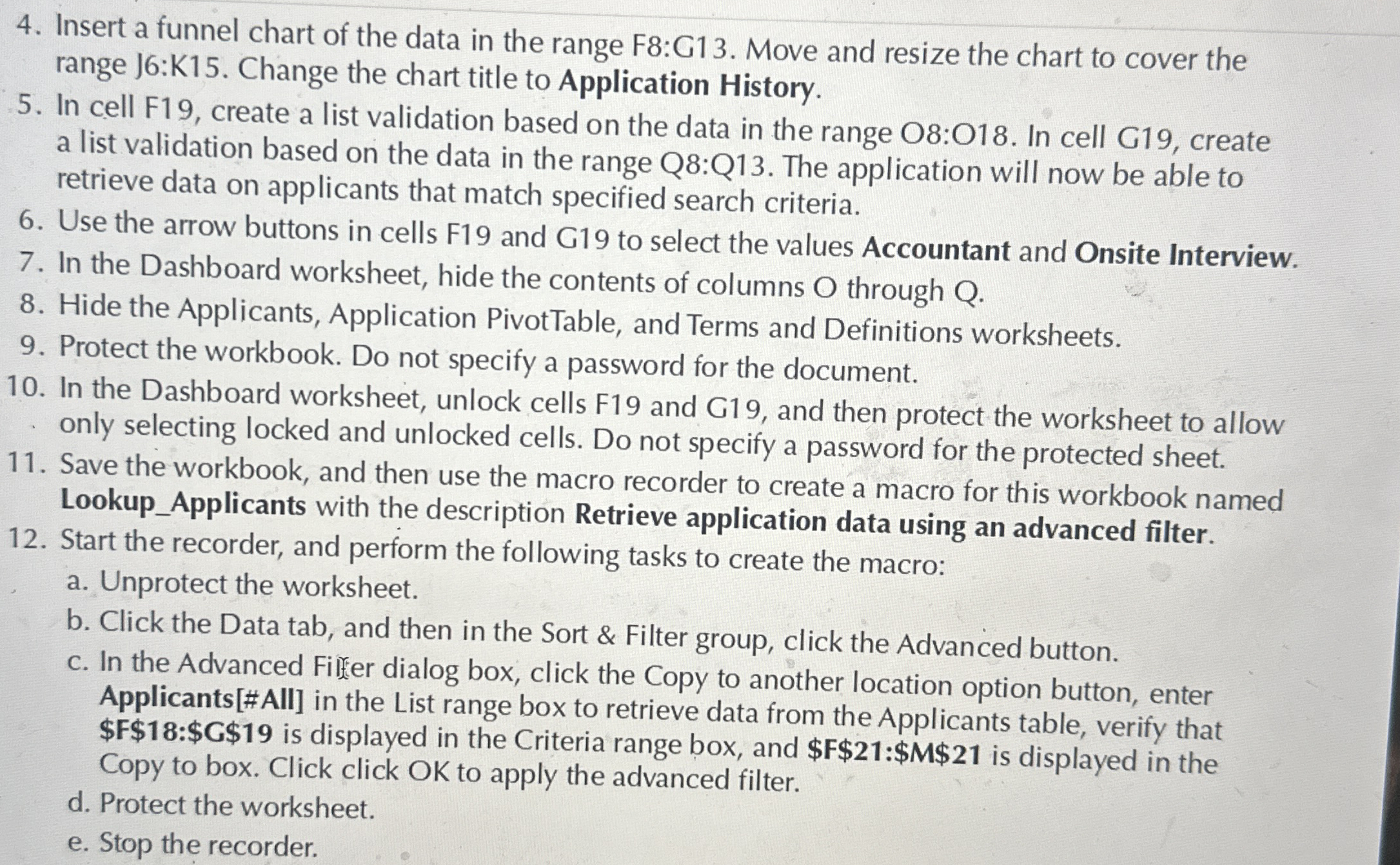
Insert a funnel chart of the data in the range F:G Move and resize the chart to cover the range J:K Change the chart title to Application History.
In cell F create a list validation based on the data in the range O:O In cell G create a list validation based on the data in the range Q:Q The application will now be able to retrieve data on applicants that match specified search criteria.
Use the arrow buttons in cells F and G to select the values Accountant and Onsite Interview.
In the Dashboard worksheet, hide the contents of columns O through Q
Hide the Applicants, Application PivotTable, and Terms and Definitions worksheets.
Protect the workbook. Do not specify a password for the document.
In the Dashboard worksheet, unlock cells F and G and then protect the worksheet to allow only selecting locked and unlocked cells. Do not specify a password for the protected sheet.
Save the workbook, and then use the macro recorder to create a macro for this workbook named LookupApplicants with the description Retrieve application data using an advanced filter.
Start the recorder, and perform the following tasks to create the macro:
a Unprotect the worksheet.
b Click the Data tab, and then in the Sort & Filter group, click the Advanced button.
c In the Advanced Filer dialog box, click the Copy to another location option button, enter Applicants#AII in the List range box to retrieve data from the Applicants table, verify that Copy to box. Click click OK to apply the advanced filter.
d Protect the worksheet.
e Stop the recorder.
Step by Step Solution
There are 3 Steps involved in it
1 Expert Approved Answer
Step: 1 Unlock

Question Has Been Solved by an Expert!
Get step-by-step solutions from verified subject matter experts
Step: 2 Unlock
Step: 3 Unlock