

Question: Mark the steps as checked when you complete them. 1 . Open the WilsonHome - 0 5 start file. If the workbook opens in Protected
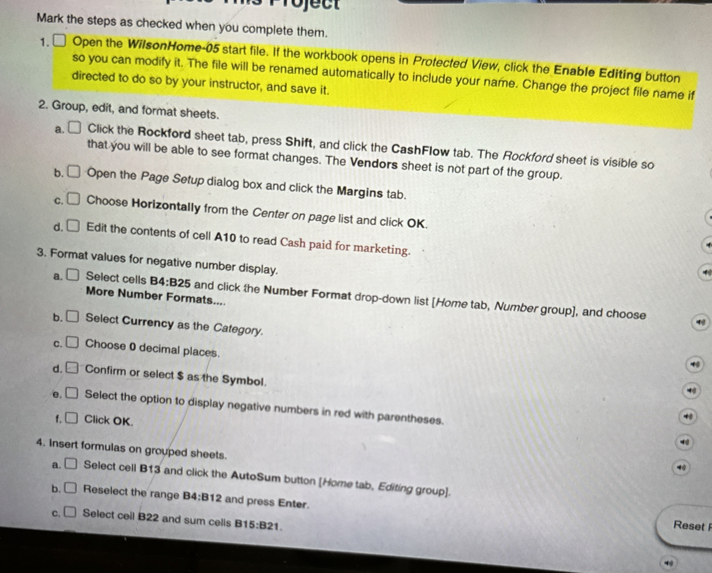
Mark the steps as checked when you complete them.
Open the WilsonHome start file. If the workbook opens in Protected View, click the Enable Editing button so you can modify it The file will be renamed automatically to include your name. Change the project file name if directed to do so by your instructor, and save it
Group, edit, and format sheets.
a Click the Rockford sheet tab, press Shift, and click the CashFlow tab. The Rockford sheet is visible so that you will be able to see format changes. The Vendors sheet is not part of the group.
b Open the Page Setup dialog box and click the Margins tab.
c Choose Horizontally from the Center on page list and click OK
d Edit the contents of cell A to read Cash paid for marketing.
Format values for negative number display.
a Select Currency as the Category.
b
c Choose decimal places.
d Confirm or select $ as the Symbol.
e Select the option to display negative numbers in red with parentheses.
f Click OK
Insert formulas on grouped sheets.
a Select cell B and click the AutoSum button Home tab, Editing group
b Reselect the range B:B and press Enter.
c Select cell B and sum cells B:B
Step by Step Solution
There are 3 Steps involved in it
1 Expert Approved Answer
Step: 1 Unlock

Question Has Been Solved by an Expert!
Get step-by-step solutions from verified subject matter experts
Step: 2 Unlock
Step: 3 Unlock