Microsoft Office 365 Excel Comprehensive 2021

Module 7 Case Problem 1

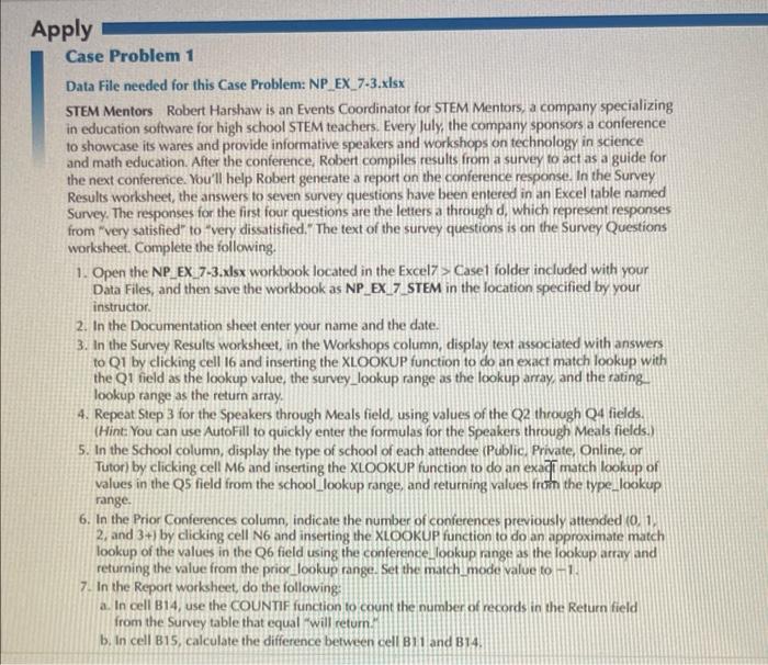
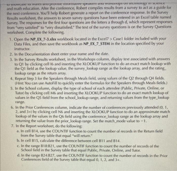
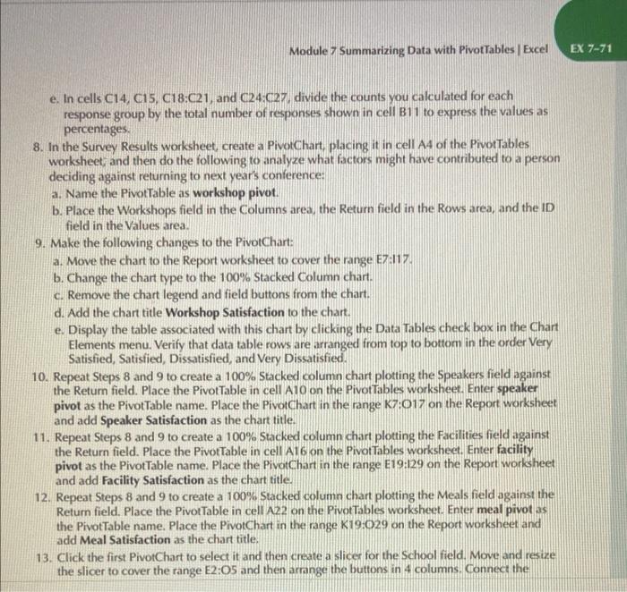
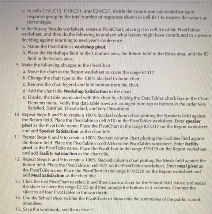
Data File needed for this Case Problem: NP_EX_7.3.xisx STEM Mentors Robert Harshaw is an Events Coordinator for STEM Mentors, a company specializing in education software for high school STEM teachers. Every luly, the company sponsors a conference to showcase its wares and provide informative speakers and workshops on technology in science and math education. After the conference, Robert compiles results from a survey to act as a guide for the next conference. You'll help Robert generate a report on the conference response. In the Survey Results worksheet, the answers to seven survey questions have been entered in an Excel table named Survey. The responses for the first four questions are the letiers a through d, which represent responses from "very satisfied" to "very dissatisfied." The text of the survey questions is on the Survey Questions worksheet. Complete the following. 1. Open the NP_EX_7-3.xlsx workbook located in the Excel7 > Casel folder included with your Data Files, and then save the workbook as NP_EX_7 STEM in the location specified by your instructor. 2. In the Documentation sheet enter your name and the date. 3. In the Survey Results worksheet, in the Workshops column, display text associated with answers to Q1 by clicking cell 16 and inserting the XLOOKUP function to do an exact match lookup with the Q1 field as the lookup value, the survey_lookup range as the lookup array, and the ratinglookup range as the return array. 4. Repeat Step 3 for the Speakers through Meals field, using values of the Q2 through Q4 fields. (Hint: You can use AutoFill to quickly enter the formulas for the Speakers through Meals fields.) 5. In the School column, display the type of school of each attendee (Public, Private, Online, or Tutor) by clicking cell M6 and inserting the XLOOKUP function to do an ext match lookup of values in the Q5 field from the school_lookup range, and returning values from the type-lookup range. 6. In the Prior Conferences column, indicate the number of conferences previously attended 10. 1. 2, and 3+1 by clicking cell N6 and inserting the XLOOKUP function to do an approximate match lookup of the values in the Q6 field using the conference lookup range as the lookup array and returning the value from the prior_lookup range. Set the match mode value to - 1 . 7. In the Report worksheet, do the following: a. In cell B14, use the COUNTIF function to count the number of records in the Return field from the Survey table that equal wwill retum? b. In cell B15, calculate the difference between cell B11 and B14. to snowcase is wares and proviue numurmative speakers and worksiops on iecmioiogy in science and math education. After the conference, Robert compiles results from a survey to act as a guide for the next conference. You'll help Robert generate a report on the conference response. In the Survey Results worksheet, the answers to seven survey questions have been entered in an Excel table named Survey. The responses for the first four questions are the letters a through d, which represent responses from "very satisfied" to "very dissatisfied." The text of the survey questions is on the Survey Questions worksheet. Complete the following. 1. Open the NP_EX_7-3.xlsx workbook located in the Excel7 > Casel folder included with your Data Files, and then save the workbook as NP_EX_7_STEM in the location specified by your instructor. 2. In the Documentation sheet enter your name and the date. 3. In the Survey Results worksheet, in the Workshops column, display text associated with answers to Q1 by clicking cell i6 and inserting the XLOOKUP function to do an exact match lookup with the Q1 field as the lookup value, the survey_lookup range as the lookup array, and the rating_lookup range as the return array. 4. Repeat Step 3 for the Speakers through Meals field, using values of the Q2 through Q4 fields. (Hint: You can use AutoFill to quickly enter the formulas for the Speakers through Meals fields.) 5. In the School column, display the type of school of each attendee (Public, Private, Online, or Tutor) by clicking cell M6 and inserting the XLOOKUP function to do an exact match lookup of values in the Q5 field from the school_lookup range, and returning values from the type_lookup range. 6. In the Prior Conferences column, indicate the number of conferences previously attended (0,1, 2 , and 3+ ) by clicking cell N6 and inserting the XLOOKUP function to do an approximate match lookup of the values in the Q6 field using the conference_lookup range as the lookup array and returning the value from the prior_lookup range. Set the match_mode value to 1. 7. In the Report worksheet, do the following: a. In cell B14, use the COUNTIF function to count the number of records in the Return field from the Survey table that equal "will return." b. In cell B15, calculate the difference between cell B11 and B14. c. In the range B18:B21, use the COUNTIF function to count the number of records of the School field in the Survey table that equal Public, Private, Online, and Tutor. d. In the range B24:B27, use the COUNTIF function to count the number of records in the Prior Conferences field of the Survey table that equal 0,1,2, and 3+. e. In cells C14, C15, C18:C21, and C24:C27, divide the counts you calculated for each response group by the total number of responses shown in cell B11 to express the values as percentages. 8. In the Survey Results worksheet, create a PivotChart, placing it in cell A4 of the PivotTables worksheet, and then do the following to analyze what factors might have contributed to a person deciding against returning to next year's conference: a. Name the PivotTable as workshop pivot. b. Place the Workshops field in the Columns area, the Return field in the Rows area, and the ID field in the Values area. 9. Make the following changes to the PivotChart: a. Move the chart to the Report worksheet to cover the range E7:117. b. Change the chart type to the 100% Stacked Column chart. c. Remove the chart legend and field buttons from the chart. d. Add the chart title Workshop Satisfaction to the chart. e. Display the table associated with this chart by clicking the Data Tables check box in the Chart Elements menu. Verify that data table rows are arranged from top to bottom in the order Very Satisfied, Satisfied, Dissatisfied, and Very Dissatisfied. 10. Repeat Steps 8 and 9 to create a 100\% Stacked column chart plotting the Speakers field against the Retum field. Place the PivotTable in cell A10 on the Pivot Tables worksheet. Enter speaker pivot as the PivotTable name. Place the PivotChart in the range K7:017 on the Report worksheet and add Speaker Satisfaction as the chart title. 11. Repeat Steps 8 and 9 to create a 100% Stacked column chart plotting the Facilities field against the Return field. Place the PivotTable in cell A1 6 on the PivotTables worksheet. Enter facility pivot as the PivotTable name. Place the PivotChart in the range E19:129 on the Report worlsheet and add Facility Satisfaction as the chart title. 12. Repeat Steps 8 and 9 to create a 100% Stacked column chart plotting the Meals field against the Retum field. Place the PivotTable in cell A22 on the Pivot Tables worksheet. Enter meal pivot as the PivotTable name. Place the PivotChart in the range K19:029 on the Report worksheet and add Meal Satisfaction as the chart title. 13. Click the first PivotChart to select it and then create a slicer for the School field. Move and resize the slicer to cover the range E2:O5 and then arrange the buttons in 4 columns. Connect the e. In cells C14,C15,C18:C21, and C24:C27, divide the counts you calculated for each response group by the total number of responses shown in cell B11 to express the values as percentages. 8. In the Survey Results worksheet, create a PivotChart, placing it in cell A4 of the PivotTables worksheet, and then do the following to analyze what factors might have contributed to a person deciding against returning to next year's conference: a. Name the PivotTable as workshop pivot. b. Place the Workshops field in the Columns area, the Return field in the Rows area, and the ID field in the Values area. 9. Make the following changes to the PivotChart: a. Move the chart to the Report worksheet to cover the range E7:117. b. Change the chart type to the 100% Stacked Column chart. c. Remove the chart legend and field buttons from the chart. d. Add the chart title Workshop Satisfaction to the chart. e. Display the table associated with this chart by clicking the Data Tables check box in the Chart Elements menu. Verify that data table rows are arranged from top to bottom in the order Very Satisfied, Satisfied, Dissatisfied, and Very Dissatisfied. 10. Repeat Steps 8 and 9 to create a 100% Stacked column chart plotting the Speakers field against the Return field. Place the PivotTable in cell A10 on the PivotTables worksheet. Enter speaker pivot as the PivotTable name. Place the PivotChart in the range K7:O17 on the Report worksheet and add Speaker Satisfaction as the chart title. 11. Repeat Steps 8 and 9 to create a 100% Stacked column chart plotting the Facilities field against the Return field. Place the PivotTable in cell A16 on the PivotTables worksheet. Enter facility pivot as the PivotTable name. Place the PivotChart in the range E19:129 on the Report worksheet and add Facility Satisfaction as the chart title. 12. Repeat Steps 8 and 9 to create a 100% Stacked column chart plotting the Meals field against the Return field. Place the PivotTable in cell A22 on the PivotTables worksheet. Enter meal pivot as the PivotTable name. Place the PivotChart in the range K19:O29 on the Report worksheet and add Meal Satisfaction as the chart title. 13. Click the first PivotChart to select it and then create a slicer for the School field. Move and resize the slicer to cover the range E2:O5 and then arrange the buttons in 4 columns. Connect the slicer to all four PivotTables in the workbook. 14. Use the School slicer to filter the PivotCharts to show only the summaries of the public school attendees. 15. Save the workbook, and then close it