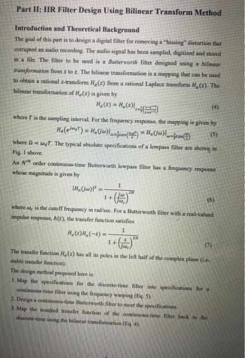
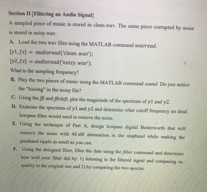
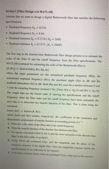
Part II: IIR Filter Design Using Bilinear Transform Method Introduction and Theoretical Background The goal of this part is to design a digital filter for removing a "hissing" distortion that comupted an audio recording. The audio signal has been sampled, digitized and stored in a file. The filter to be used is a Butterworth filter designed using a bilineur transformation from s to 2 . The bilinear transformation is a mapping that can be used to obtain a national 2-transform Hd(z) from a rational Laplace transform Ha (s). The bilinear transformation of Ha(s) is given by Hd(z)=Ha(s)s=T(1+z11z1) where T is the sampling interval. For the frequency response, the mapping is given by Ha(ejdT)=Ha(j)=Ttan(2a)=Ha(f)=r2tan(2) where =dT. The typical absolute specifications of a lowpass filter are shown in Fig. 1 above. An Nth order continuous-time Butterworth lowpass filter has a frequency response: whose magnitude is given by Ha(j)2=1+(jcj)2N1 Where c is the cutoff frequency in rad/see. For a Butterworth filter with a real-valued impulse response, h(t), the transfer function satisfies Ha(s)Ha(s)=1+(cs)2N1 The transfer function Ha(s) has all its poles in the left half of the complex plane (i.e., stable transfer function). The design method proposed here is: 1. Map the specifications for the disereto-time filter into specifications for a continuous-time filter using the frequency warping (Eq 5). 2. Derign a continuous-time Butterworth filter to meet the specificationi. 3. Map the resulied trander function of the continuous-time filer back to the diserete-time using the bilinear transformation (Eq,4). Section II [Filtering an Audio Signal] A sampled piece of music is stored in clean.wav. The same piece corrupted by noise is stored in noisy.wav. A. Load the two wav files using the MATLAB command wavread. [y1,fs]=audioread(clean.wav)[y2,fs]=audioread(noisy.wav) What is the sampling frequency? B. Play the two pieces of music using the MATLAB command sound. Do you notice the "hissing" in the noisy file? C. Using the ff and ff shift, plot the magnitude of the spectrum of y1 and y2. D. Examine the spectrum of y1 and y2 and determine what cutoff frequency an ideal lowpass filter would need to remove the noise. E. Using the technique of Part A, design lowpass digital Butterworth that will remove the noise with 40dB attenuation in the stopband while making the passband ripple as small as you can. F. Using the designed filter, filter the data using the filter command and determine how well your filter did by: 1) listening to the filtered signal and comparing its quality to the original one and 2) by comparing the two spectra. Section I [Filter Design a la MATLAB] Assume that we want to design a digital Butterworth filter that satisfies the following specifications: - Passband frequency p=0.22. Stopband frequency s=0.4. - Passband tolerance p=0.1710(Rp=3dB) - Poissband tolerance s=0.1171(As=20dB) The first step in the discrete-time Butterworth filter design process is to estimate the order of the filter N and the cutoff frequency from the filter specifications. The MATLAB command for estimating the order of the Butterworth filier is [N,Wc]=buttord(Wp,Ws,Rp,As) where the inpat parameters are the normalized passband frequency (Wp), the nomalized stopband frequency (Ws), the passband ripple (Rp) in dB and the Topband attenuation (As) in dB. Both Wp and Ws must be a number between 0 and 1 with the sampling frequency assumed 2Hz. [Note: Wp=p/ and Ws=3/ ] The output data are the lowest order N meeting the specifications and the cutoff frequency. After the filter order and the cutoff frequency have been estimated, the ned step is to determine the transfer function of the filter. This is done using the command [num,den] = butter (N,Wc) where num and den contain, respectively, the coefficients of the numerator and denominator polynomials of transfer function in ascending powers if 21. A. What are: i) the otder of the filter and ii) the cutoff frequency 8. Write the transfer function of the discrete-time Butterworth filter. C. Use plane command in MATLAB to plot the zeros and poles of the discrete-time filter, Is the filter stable or unstable? D. Using MATLAB command freqz, plot the magnitude and the phase of the froquency reyonie of the digital fiter. Does the magnitude reuponse satiufy the Mpecificitione if not, what may be the reasons? 1. In the phuse reapotse linear within the pawband? If ost, what musy be the rosoon