Please Answer in MATLAB Code (not by hand)

Question:

Reference Material:

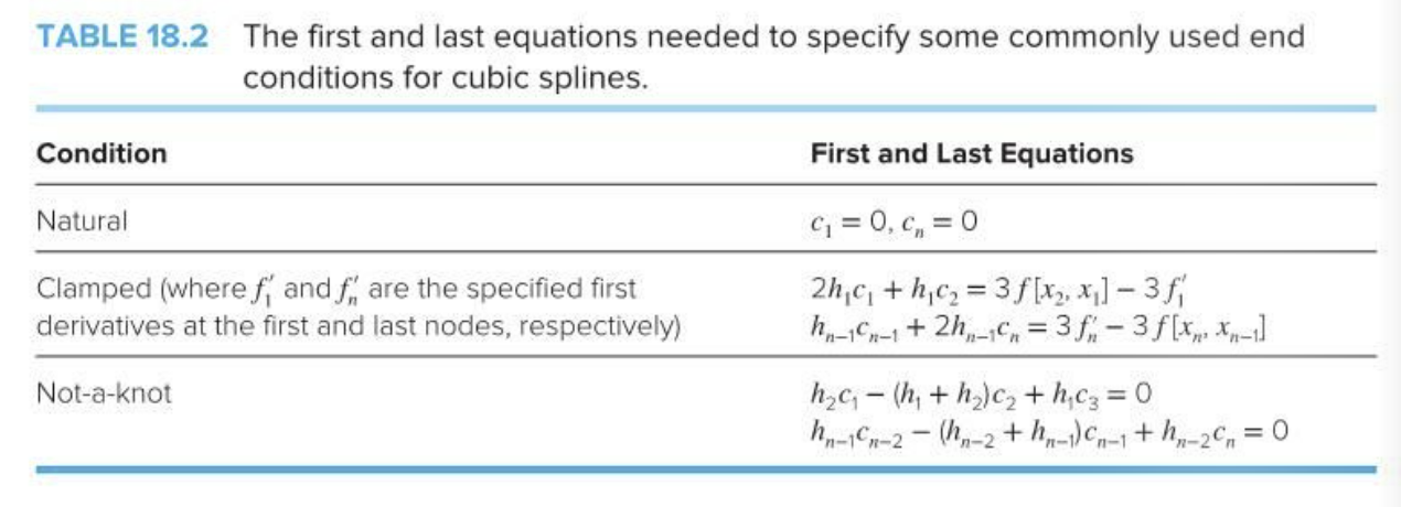
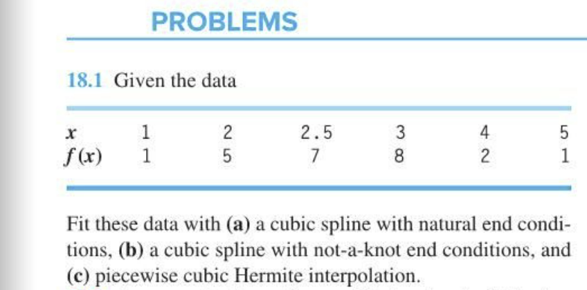
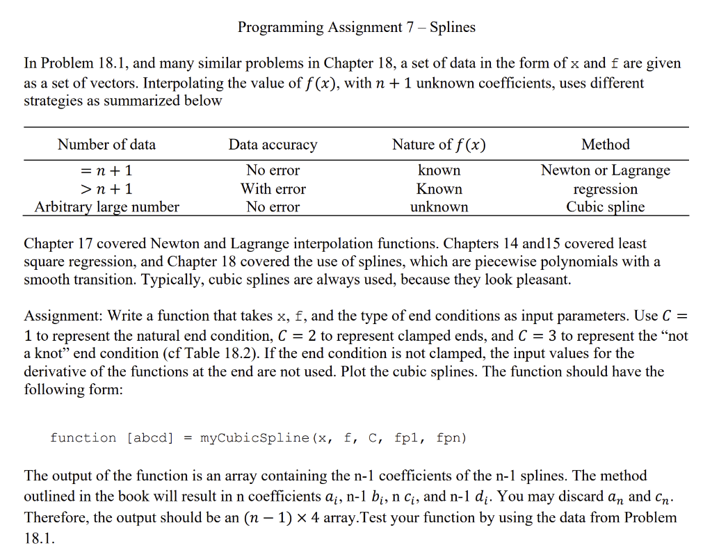
In Problem 18.1, and many similar problems in Chapter 18 , a set of data in the form of x and f are given as a set of vectors. Interpolating the value of f(x), with n+1 unknown coefficients, uses different strategies as summarized below Chapter 17 covered Newton and Lagrange interpolation functions. Chapters 14 and 15 covered least square regression, and Chapter 18 covered the use of splines, which are piecewise polynomials with a smooth transition. Typically, cubic splines are always used, because they look pleasant. Assignment: Write a function that takes x,f, and the type of end conditions as input parameters. Use C= 1 to represent the natural end condition, C=2 to represent clamped ends, and C=3 to represent the "not a knot" end condition ( cf Table 18.2). If the end condition is not clamped, the input values for the derivative of the functions at the end are not used. Plot the cubic splines. The function should have the following form: function[abcd]=myCubicSpline(x,f,c,fpl,fpn) The output of the function is an array containing the n1 coefficients of the n1 splines. The method outlined in the book will result in n coefficients ai,n1bi,nci, and n1di. You may discard an and cn. Therefore, the output should be an (n1)4 array.Test your function by using the data from Problem 18.1. TABLE 18.2 The first and last equations needed to specify some commonly used end conditions for cubic splines. Fit these data with (a) a cubic spline with natural end conditions, (b) a cubic spline with not-a-knot end conditions, and (c) piecewise cubic Hermite interpolation. In Problem 18.1, and many similar problems in Chapter 18 , a set of data in the form of x and f are given as a set of vectors. Interpolating the value of f(x), with n+1 unknown coefficients, uses different strategies as summarized below Chapter 17 covered Newton and Lagrange interpolation functions. Chapters 14 and 15 covered least square regression, and Chapter 18 covered the use of splines, which are piecewise polynomials with a smooth transition. Typically, cubic splines are always used, because they look pleasant. Assignment: Write a function that takes x,f, and the type of end conditions as input parameters. Use C= 1 to represent the natural end condition, C=2 to represent clamped ends, and C=3 to represent the "not a knot" end condition ( cf Table 18.2). If the end condition is not clamped, the input values for the derivative of the functions at the end are not used. Plot the cubic splines. The function should have the following form: function[abcd]=myCubicSpline(x,f,c,fpl,fpn) The output of the function is an array containing the n1 coefficients of the n1 splines. The method outlined in the book will result in n coefficients ai,n1bi,nci, and n1di. You may discard an and cn. Therefore, the output should be an (n1)4 array.Test your function by using the data from Problem 18.1. TABLE 18.2 The first and last equations needed to specify some commonly used end conditions for cubic splines. Fit these data with (a) a cubic spline with natural end conditions, (b) a cubic spline with not-a-knot end conditions, and (c) piecewise cubic Hermite interpolation