PLEASE MAKE AURE IT IS NOT BLURRY.

every other answer to this question is too blurry to view.

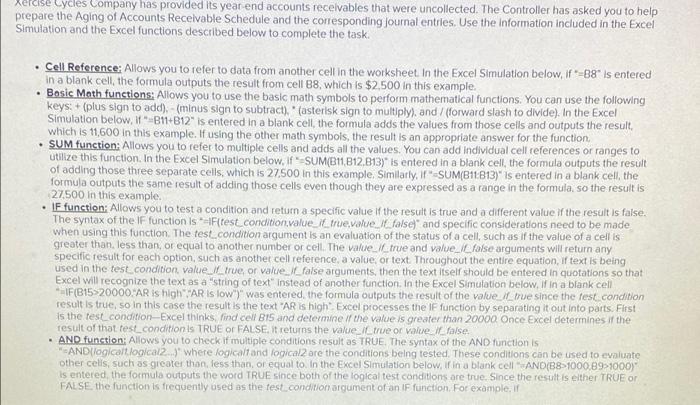
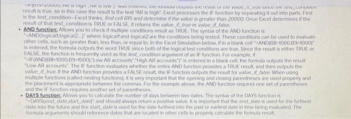
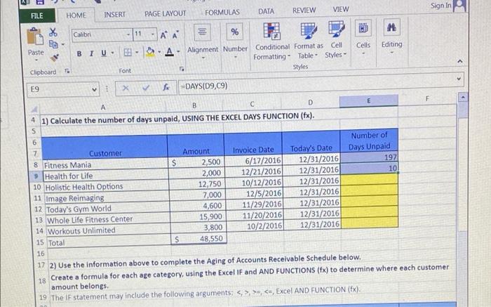
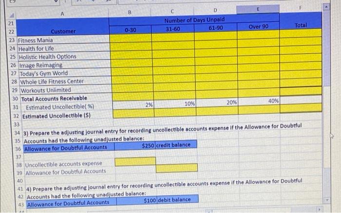
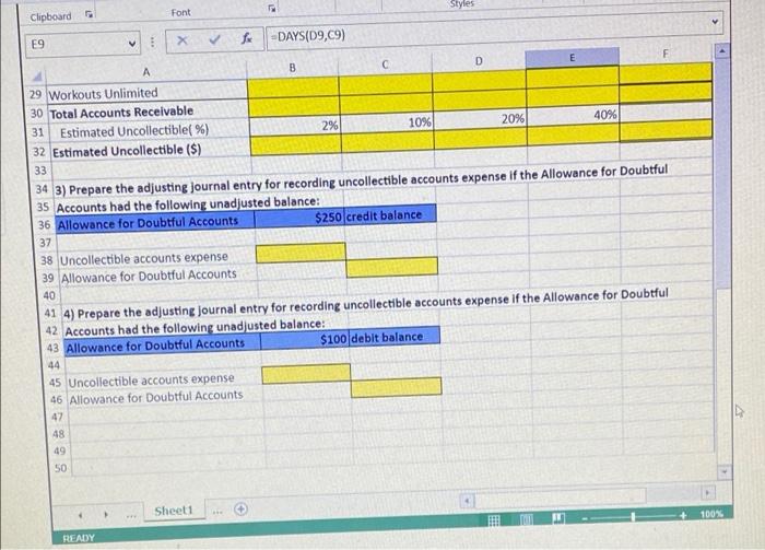
Xercise Cycles Company has provided its year end accounts receivables that were uncollected. The Controller has asked you to help prepare the Aging of Accounts Receivable Schedule and the corresponding Journal entries. Use the Information included in the Excel Simulation and the Excel functions described below to complete the task. Cell Reference: Allows you to refer to data from another cell in the worksheet in the Excel Simulation below, if-88" is entered in a blank cell, the formula outputs the result from cell B8, which is $2.500 in this example. Basic Math functions: Allows you to use the basic math symbols to perform mathematical functions. You can use the following keys: + (plus sign to add) (minus sign to subtract), " (asterisk sign to multiply), and / (forward slash to divide). In the Excel Simulation below, 11"-311-B12" is entered in a blank cell, the formula adds the values from those cells and outputs the result, which is 11,600 in this example. If using the other math symbols, the result is an appropriate answer for the function SUM function: Allows you to refer to multiple cells and adds all the values. You can add individual cell references or ranges to utilize this function. In the Excel Simulation below. If SUM(B11, B12,813)" is entered in a blank cell, the formula outputs the result of adding those three separate cells, which is 27.500 in this example, Similarly, if SUM(B11813)" is entered in a blank cell, the formula outputs the same result of adding those cells even though they are expressed as a range in the formula, so the result is 27500 in this example, IF function: Allows you to testa condition and return a specific value of the result is true and a different value if the result is false. The syntax of the IF function is --F{test condition value_it_true value. Ifalse)" and specific considerations need to be made when using this function. The test condition argument is an evaluation of the status of a cell, such as if the value of a cellis greater than less than or equal to another number or cell. The value. I true and value_ I false arguments will return any specific result for each option, such as another cell reference, a value or text. Throughout the entire equation of text is being used in the test condition value Il true or value_l_false arguments, then the text itself should be entered in quotations so that Excel will recognize the text as a "string of text" instead of another function in the Excel Simulation below. If in a blank cell IF(B1520000. AR is high" PARIS low") was entered the formula outputs the result of the value_l_mue since the test condition result is true, so in this case the result is the text "AR is high". Excel processes the IF function by separating it out into parts. First is the test condition-Excel thinks, find cell BTS and determine if the value is greater than 20000 Once Excel determines if the result of that test condition is TRUE OR FALSE It returns the value_true or wwwe. Il false AND function: Allows you to check if multiple conditions result as TRUE The syntax of the AND function is "AND logical local2..) where logical and logical2 ore the conditions being tested. These conditions can be used to evaluate other cells, such as greater thon, less than or equal to in the Excel Simulation below, if in a blank cell" AND(B8>1000.89>1000) Is entered the formula outputs the word TRUE since both of the logical test conditions are true. Since the result is either TRUE OR FALSE, the function is frequently used as the rest.condition argument of an IF function. For example, if -615 ZVU, ARISTARSTOW Was H, WIE IOUIS VULPULSUITES UUE VareILUSIEURILOR result is true, so in this case the result is the text "AR is high". Excel processes the IF function by separating it out into parts. First is the test. condition-Excel thinks, find cell B15 and determine if the value is greater than 20000 Once Excel determines if the result of that test condition is TRUE OR FALSE It returns the value. (true or value false AND function: Allows you to check if multiple conditions result as TRUE. The syntax of the AND function is **AND(logicaltlogical2) where logical and logical are the conditions being tested. These conditions can be used to evaluate other cells, such as greater than less than or equal to in the Excel Simulation below. If in a blank cell-AND(88-1000,89-1000) Is entered the formula outputs the word TRUE since both of the logical test conditions are true. Since the result is either TRUE ON FALSE, the function is frequently used as the test condition argument of an IF function. For example, if "IF(AND(B8>1000,89-1000). "Low AR accounts High AR accounts")" is entered in a blank cell, the formula outputs the result *Low AR accounts The IF function evaluates whether the entire AND function provides a TRUE result and then outputs the value_true. If the AND function provides a FALSE result, the IF function outputs the result for value falseWhen using multiple functions (called nesting functions). It is very important that the opening and closing parentheses are used property and the placement is appropriate between the commas. For the example above, the AND function requires one set of parentheses and the IF function requires another set of parentheses DAYS function: Allows you to calculate the number of days between two dates. The syntax of the DAYS function is =DAYS(end date start date and should always return a positive value. It is important that the end date is used for the furthest date into the future and the start date is used for the date furthest into the past or earliest date in time being evaluated. The formula arguments should reference dates that are located in other cells to properly calculate the formula result, VIEW Sign In FILE HOME INSERT REVIEW PAGE LAYOUT FORMULAS DATA > M m. Win Calibri - 11 EC Paste Cells Editing BIU - -AA % SA - Alignment Number Conditional Format as Cell Formatting - Table - Styles - Styles . Font Clipboard E9 X fc-DAYS(D9,09) . A B C D 4 1) Calculate the number of days unpaid, USING THE EXCEL DAYS FUNCTION (fx). S 6 Number of 7 Customer Amount Invoice Date Today's Date Days Unpaid 8 Fitness Mania S 2,500 6/17/2016 12/31/2016 1971 9 Health for Life 2,000 12/21/2016 12/31/2016 10 10 Holistic Health Options 12,750 10/12/2016 12/31/2016 11 Image Reimaging 7,000 12/5/2016 12/31/2016 12 Today's Gym World 4,600 11/29/2016 12/31/2016 13 Whole Life Fitness Center 15,900 11/20/2016 12/31/2016 14 Workouts Unlimited 3,800 10/2/2016 12/31/2016 15 Total S 48,550 16 17 2) Use the information above to complete the Aging of Accounts Receivable Schedule below. 18 Create a formula for each age category, using the Excel IF and AND FUNCTIONS (4x) to determine where each customer amount belongs 19 The IF statement may include the following arguments: >