please use excel and show all steps/ equations!!!

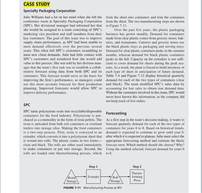
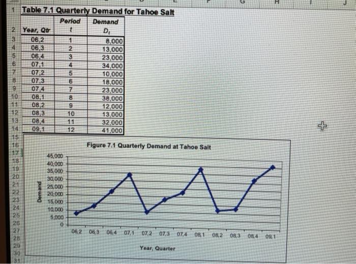
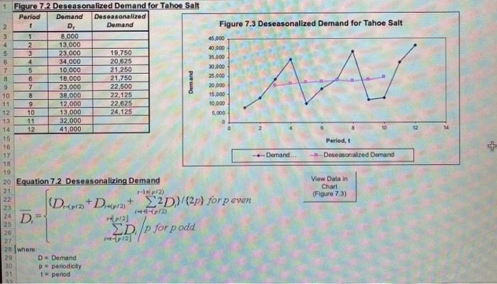
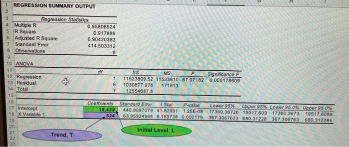
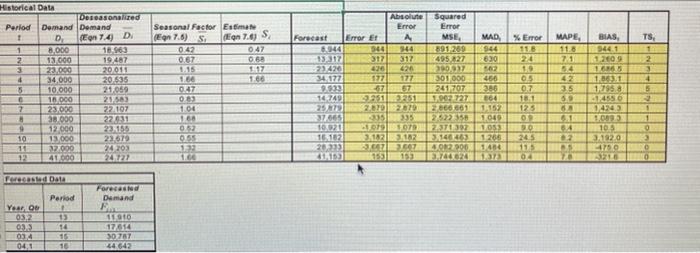
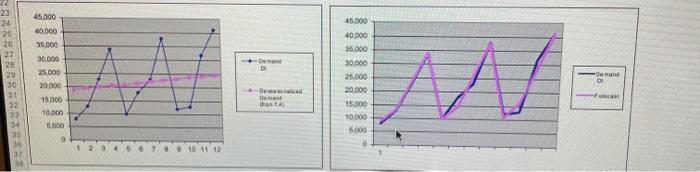
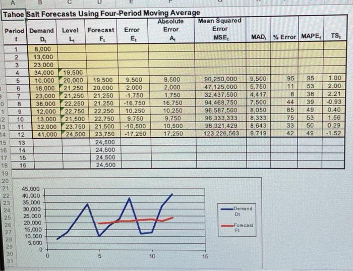
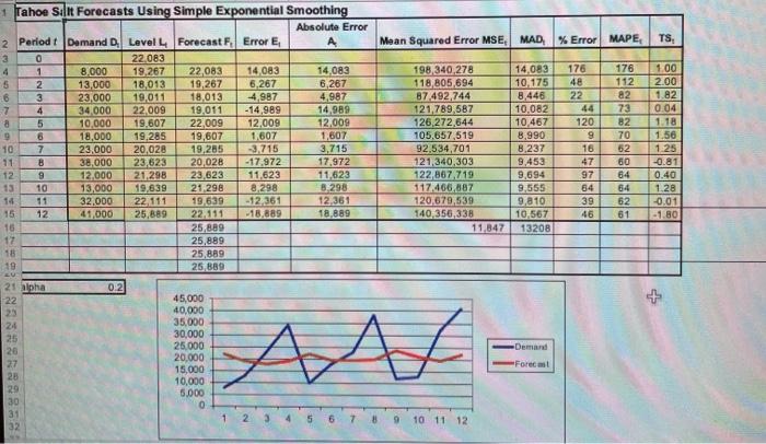
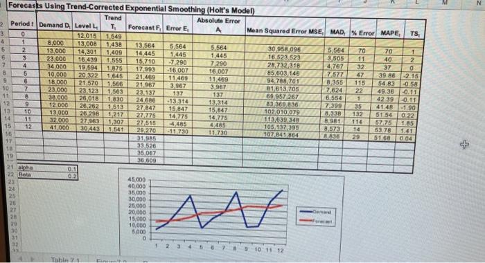
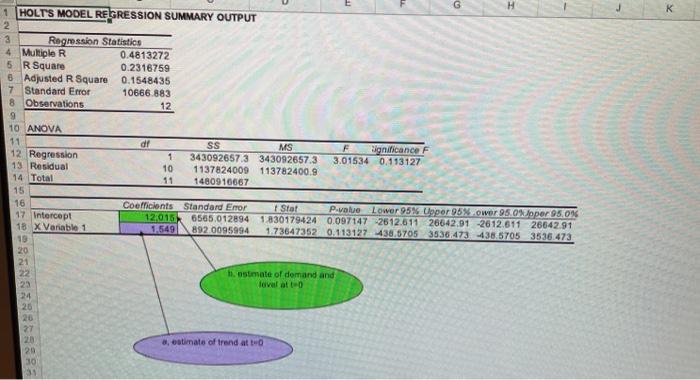
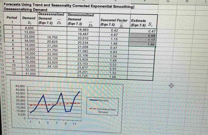
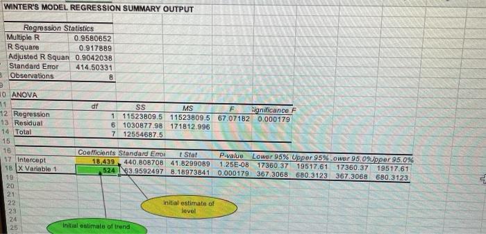
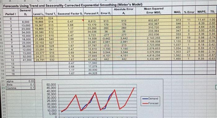
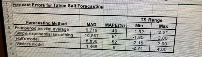
CASE STUDY Specialty Packaging Corporation Julie Williams had a lot on her mind when she left the form the sheet into containers and trim the containers conference room at Specialty Packaging Corporation from the sheet. The two manufacturing steps are shown (SPC). Her divisional manager had informed her that in Figure 7-11. she would be assigned to a team consisting of SPC's Over the past five years, the plastic packaging marketing vice president and staff members from their business has grown steadily. Demand for containers key customers. The goal of this team was to improve made from clear plastic comes from grocery stores, bak- supply chain performance, as SPC had been unable to eries, and restaurants. Caterers and grocery stores use meet demand effectively over the previous several the black plastic trays as packaging and serving trays. years. This often left SPC's customers scrambling to Demand for clear plastic containers peaks in the summer meet new client demands. Julie had little contact with months, whereas demand for black plastic containers SPC's customers and wondered how she would add peaks in the fall. Capacity on the extruders is not suffi- value to this process. She was told by her division man- cient to cover demand for sheets during the peak sea- ager that the team's first task was to establish a collab- sons. As a result, the plant is forced to build inventory of orative forecast using data from both SPC and its each type of sheet in anticipation of future demand. customers. This forecast would serve as the basis for Table 7-4 and Figure 7-12 display historical quarterly improving the firm's performance, as managers could demand for each of the two types of containers (clear use this more accurate forecast for their production and black). The team modified SPC's sales data by planning. Improved forecasts would allow SPC to accounting for lost sales to obtain true demand data. improve delivery performance. Without the customers involved in this team, SPC would never have known this information, as the company did not keep track of lost orders. SPC SPC turns polystyrene resin into recyclable/disposable containers for the food industry. Polystyrene is pur- Forecasting chased as a commodity in the form of resin pellets. The As a first step in the team's decision making, it wants to resin is unloaded from bulk rail containers or overland forecast quarterly demand for each of the two types of trailers into storage silos. Making the food containers containers for years 6 to 8. Based on historical trends, is a two-step process. First, resin is conveyed to an demand is expected to continue to grow until year 8. extruder, which converts it into a polystyrene sheet that after which it is expected to plateau. Julie must select the is wound into rolls. The plastic comes in two forms appropriate forecasting method and estimate the likely clear and black. The rolls are either used immediately forecast error. Which method should she choose? Why? to make containers or put into storage. Second, the Using the method selected, forecast demand for years 6 rolls are loaded onto thermoforming presses, which to 8. Step 1 Step 2 Thermo- forming Press Resin Extruder Roll Storage Storage FIGURE 7-11 Manufacturing Process at SPC This is a challenging case study where you have to select an appropriate forecasting method and use the method to forecast the demand for quarters I, II, III and IV for years 6 to 8. Instead of starting from scratch, I recommend that you modify the Tahoe Salt excel model. The text explains in detail how different forecasting methods were applied to the Tahoe Salt. Read the text before modifying the Tahoe Salt file. For your convenience, a copy of the Tahoe Salt excel file has been uploaded in this module. 07.4 Table 7.1 Quarterly Demand for Tahoe Salt Period Demand 2 Year, Qor D. 06.2 1 8,000 06,3 2 13,000 06.4 3 23,000 6 07,1 4 34,000 072 5 10,000 8 07.3 6 18,000 7 23,000 10 08.1 8 38.000 11 082 9 12,000 12 08,3 10 13,000 13 08,4 11 32,000 14 09.1 12 41,000 15 16 Figure 7.1 Quarterly Demand at Tahoe Salt 45,000 40,000 19 35,000 20 30.000 21 25.000 22. 20.000 23 15.000 24 10.000 25 5.000 26 0 27 062 06,3 064 07,1 072 07.3 07.4 081 28 082 083 29 Year, Quarter 30 084 091 Figure 7.3 Deseasonalized Demand for Tahoe Salt 1 Fiqure 72 Deseasonalized Demand for Tahoe Salt Period Demand Deseasonalized 2 D Demand 3 5 8,000 4 2 13,000 5 3 23,000 19,750 6 4 34,000 20.825 7 5 10.000 21.250 8 6 18.000 21.750 7 23,000 22,500 10 8 38,000 22.125 11 9 12,000 22.625 12 10 13,000 24.125 13 11 32,000 14 12 41,000 Demand 45.000 40.000 35.000 30,000 25.000 20.000 15.000 10.000 5.000 10 14 Period, t st -Demand... Deseasonalized Demand 16 17 18 19 20 Equation 7.2 Deseasonalizing Demand 21 -1/2) 22 + View Data in Chart (Figure 7.3) Dev+D 2D}(2p) for p even ID /pfor for podd 24 D 25 26 27 28 where 29 D = Demand 30 - periodicity 31 1 - period 1 REGRESSION SUMMARY OUTPUT 2 3 3 Regression Statistics 4 Multiple 0.95806524 5 R Square 0.917889 6 Adjusted R Square 0.90420383 Standard Error 414.503312 8 Observations 8 9 10 ANOVA 11 df 12 Regression 1 13 Residual 6 14 Total 7 15 16 Coefficients 17 Intercept 18.439 18 X Variable 1 524 19 20 21 Trend, T 22 23 SS MS F 11523809.52 11523810 67.07182 1030877.976 171813 125546875 Significance E 0.000178609 Standard Error Star P-value Lower 95% Upper 95% Lower 95.0% Upper 95.0% 440.8087079 41.82991 1256-08 17360.36726 19517.609 17360.3673 19517.6089 63 95924968 8.189738 0.000179 367 3067633 680.31228 387 306783 680.312284 Initial Level, L En ZS Emor BIAS, Seasonal Factor Esmer En 7.6) 042 047 0.67 08 8.15 1.66 16 MAPE, 110 71 1.2009 Historical Data Deseasonalid Perlod Demand Demand 1 D, Eos 7.4 D 1 8.000 18.963 2 13 000 19487 3 23,000 20011 4 34.000 20.535 5 10.000 21.059 6 16.000 2153 7 23.000 224107 8 35 000 22631 9 12 000 23.155 10 13,000 23.679 12.000 24203 12 41.000 20122 Absolute Squared Error Error Forecast Error Er A MSE, MAD 044 544 891 200 13317 317 317 495 27 630 73420 426 420 2007 34,177 177 177 301 000 241707 16749 164 2572 2010 2019 2666667814157 37065 305 3.35 12522350 1.049 1021 Toto SOT IZS71053 16182 3.182 3.182 20333 3507 0290021484 2013 TS, 1 2 3 4 5 OS 0.7 1.8631 1.295.0 114550 14243 083 104 16 42 35 5. 63 6.1 84 02 35 09 1 1 0 055 245 193 10.15 3.1920 4790 23210 16 O Forecast Data Period Foreca Demand E 11 10 Year On 032 0:35 014 041 16 30287 14642 45.000 45.000 40,000 35.000 40.000 23 24 25 20 27 28 20 30 31 De 10 H 30.000 25.000 20.000 15.000 10.000 3.000 35.000 30.000 25,000 20.000 15.000 10.000 5.000 / D Det 33 34 35 30 37 O B TS 1.00 2.00 2.21 -0.93 0.40 1.56 0.29 -1.52 Tahoe Salt Forecasts Using Four-Period Moving Average Absolute Mean Squared Period Demand Level Forecast Error Error Error t D F EL MSE, MAD, % Error MAPE, 1 8,000 2 13,000 3 23,000 4 34,000 19,500 5 10,000 20.000 19,500 9,500 9,500 90,250.000 9,500 95 95 6 18,000 21,250 20,000 2.000 2.000 47 125,000 5.750 11 53 3 7 23,000 21,250 21.250 -1.750 1,750 32.437,500 4,417 8 38 0 8 38,000 22,250 21,250 -16.750 16.750 94.468,750 7,500 44 39 1 9 12.000 22.750 22.250 10,250 10.250 96,587,500 8,050 85 49 12 10 13,000 21,500 22.750 9.750 9.750 96,333,333 8,333 75 53 13 11 32,000 23.750 21,500 -10,500 10,500 98,321,429 8.643 33 50 14 41,000 24.500 23,750 -17.250 17.250 123 226,563 9,719 42 49 15 24,500 16 14 24,500 17 15 24,500 18 16 24,500 19 20 21 45,000 22 40.000 23 35,000 24 30,000 Demand 25 25,000 DI 26 20.000 Forecast 27 15,000 FI 10,000 28 5,000 0 30 0 5 10 31 15 12 13 TS, 1 Tahoe Silit Forecasts Using Simple Exponential Smoothing Absolute Error 2 Period t Demand D Level L Forecast F. Error E A Mean Squared Error MSE, MAD, % Error MAPE, 3 0 22,083 4 1 8.000 19,267 22,083 14,083 14.083 198 340 278 14,083 176 176 5 2 13,000 18,013 19,267 6,267 6,267 118,805 694 10,175 48 112 6 3 23,000 19,011 18,013 4,987 4.987 87.492,744 8,446 22 82 7 4 34.000 22.009 19.011 -14,989 14,989 121,789,587 10,082 73 8 5 10,000 19,607 22.009 12.009 12.009 126,272,644 10.467 120 82 9 6 18,000 19,285 19,607 1,607 1,607 105.657,519 8,990 9 70 10 7 23,000 20,028 19,285 -3,715 3,715 92,534,701 8.237 16 62 11 B 38,000 23,623 20,028 - 17.972 17,972 1121,340.303 9,453 47 60 12 9 12.000 21.298 23,623 11,623 11.623 122 867 719 9,694 97 64 13 10 13,000 19.639 21 298 8,298 8.298 117.466.887 9.555 54 64 14 11 32.000 22 111 19.639 -12,361 12,361 120,679,539 9,810 39 62 15 12 41,000 25,889 22.111 -18.889 18,889 140,356,338 10.567 46 61 16 25,889 11,847 13208 17 25,889 18 25,889 19 25 889 LU 2 1 pha 0.2 22 45,000 25 40,000 24 35,000 25 30,000 26 25.000 -Demand 20,000 27 15,000 Forecast 25 29 10,000 5.000 30 31 1 2 32 5 6 7 8 9 10 11 12 1.00 2.00 1.82 0.04 1.18 1.56 1.25 -0.81 0.40 1.28 -0.01 -1.80 $ H N Forecasts Using Trend-Corrected Exponential Smoothing (Holt's Model) Trend Absolute Error 2 Period t Demand D Level L T Forecast F. Error E A Mean Squared Error MSE, MAD, % Error MAPE, TS 3 0 12,015 1,549 4 1 8.000 13,008 1438 13,564 5,564 5,564 30,958,096 5,564 5 70 2 1 13 000 70 14,3011,409 14 445 1,445 1.445 6 16,523 523 3 11 3,505 40 2 23.000 16,439 1.555 15.710 -7290 7,290 28,732,318 2 4 4,767 32 0 37 34 000 19,594 1.875 17.993 -16.007 16 007 8 85,603 146 7,577 47 5 10,000 20.322 39 A6 -2.15 1,645 21.469 9 11.469 11 469 94, 788,701 6 18.000 8.355 115 5483 0.58 21,570 1,566 21,967 3.967 3.967 10 81,613,705 7 23,000 7,624 22 49.38 23.123 1,563 -0.11 23.137 137 137 69,957,267 11 38.000 6.554 8 1 26,018 1,830 24 686 42.39-0.11 -13 314 13314 12 33369.236 9 12 000 7.399 35 26 262 41.48 1513 27 847 15 847 -1.90 15,847 13 102010.0792 10 13,000 20298 1,217 0,338 132 51.54 0.22 27.775 14.775 14.775 113,639,348 14 11 32 000 8,981 114 27,963 57 75 1.307 1.85 27,515 4485 15 12 41,000 105137395 8,573 14 30 443 1,541 29270 53.78 1.41 -11.730 11.730 107,841 884 15 8,836 29 5160 0.04 31,985 17 33.526 10 35,067 19 36,609 21 ha 22 Rota 0 45.000 25 40,000 24 35,000 30,000 20 25.000 27 20,000 28 15.000 30 10.000 30 5.000 0 33 7 10 11 12 Tabin G 1 HOLTS MODEL REGRESSION SUMMARY OUTPUT 2 3 Regmssion Statistics 4 Multiple R 0.4813272 5 R Square 0.2316759 8 Adjusted R Square 0.1548435 7 Standard Error 10666.883 8 Observations 12 9 10 ANOVA 11 dr SS MS F Significance F 12 Regression 1 343092657.3 343092657.3 3.01534 0.113127 13 Residual 10 1137824009 113782400.9 14 Total 11 1480916667 15 16 Coeficients Standard Emor 1 Stat P.valve Lower 95% Upper 95%ower 95.0per 95.0% 17 Intercept 12:015 6565.012894 1.830179424 0.097147-2612.611 26642.91 -2612.611 26642.91 18 x Variable 1 1.549 892 0095994 1.73647352 0.113127 438.5705 3536,473 438.5705 3536.473 19 20 21 22 1. estimate of demand and 23 level att 24 26 20 27 20 8, estimate of trend at two 20 30 G (Eqn 7.6) S 0.47 0.68 1.17 1.66 Forecasts Using Trend and Seasonality Corrected Exponential Smoothing) Deseasonalizing Demand Deseasonalized Deseasonalized Period Demand Demand Demand Seasonal Factor Estimate 3 1 D (Egn 7.2) D (Eqn 7.3) D (Egn 7.5) S. 1 1 8,000 18,963 0.42 5 2 13,000 19,487 0.67 6 3 23,000 19,750 20,010 1.15 7 4 34,000 20,625 20,534 1.66 8 5 10,000 21,250 21.058 0.47 9 6 18,000 21,750 21,582 10 0.83 7 23,000 22,500 22,106 1.04 11 8 38,000 22.125 22,629 1.68 12 9 12,000 22,625 23,153 13 0.52 10 13,000 24 125 23,677 14 0.55 11 32.000 24,201 15 12 1.32 41,000 24,725 16 1.66 17 18 45,000 19 40,000 20 35,000 30,000 Demand 22 25,000 23 20,000 24 15,000 --Deseasonized 25 10,000 Demand 5,000 27 0 20 3 7 9 11 29 30 + 21 AV 5 WINTER'S MODEL REGRESSION SUMMARY OUTPUT Regression Statistics Multiple R 0.9580652 R Square 0.917889 Adjusted R Squar 0.9042038 Standard Error 414.50331 8 Observations df SS MS F Significance F 1 11523809.5 11523809.5 67.07182 0.000179 61030877.98 171812.996 7 12554687.5 10 ANOVA 11 12 Regression 13 Residual 14 Total 15 16 17 Intercept 1 X Variable 1 19 20 21 22 23 24 25 Coefficients Standard Emi Star 18,439 440.808708 41.8299089 524 63.9592497 8.18973841 P-value Lower 95% Upper 95% .ower 95.0%Upper 95.0% 1.25E-OB 17360.37 19517,61 17360.37 19517.61 0.000179 367.3068 680.3123 367.3068 680.3123 initial estimate of level initial estimate of trend MAD, % Error MAPE, TS, 512 913 546 450 347 333 851 1,155 1,037 1,054 1,303 1,562 1.469 11 1 1 0 3 19 13 1 10 27 13 1 Forecasts Using Trend and Seasonality Corrected Exponential Smoothing (Winter's Model) Demand Absolute Error Mean Squared Period D Level L Trend T, Seasonal Factor Forecast F. Error E A Error MSE, 0 18,439 524 1 1 8,000 18.866 514 0.47 8,913 913 913 832,857 5 2 13,000 19,367 513 0.68 13,179 179 179 432 367 3 23,000 19,869 512 1,17 23,260 260 260 310.720 7 4 34.000 20,380 1.67 34,036 36 36 233,364 8 5 10,000 20.921 515 0.47 9,723 -277 277 202.036 9 6 18.000 21.689 540 0.68 14,558 3442 3.442 2,143,255 10 7 23,000 22,102 527 25,981 2.981 2.981 3,106,508 11 8 38.000 22.636 528 1.67 37,787 -213 213 2.723,856 12 9 12.000 23,291 541 0.47 10 810 -1,190 1.190 2.578,653 13 10 13,000 23.577 515 0.69 16,544 3,544 3,544 3,576,894 14 11 32.000 24.271 533 1.16 27.849 -4.151 4.151 4,818,258 15 12 41,000 24,791 532 41.442 442 442 4.432,987 16 13 0.47 11,940 17 14 0.68 17,579 18 15 1.17 30.930 19 16 1.67 44,928 20 21 alpha 0.05 22 Bota 0.1 50,000 23 Gamma 0.1 45,000 24 40,000 25 35.000 30,000 27 25,000 -Demand 28 20,000 -Forecast 29 15,000 30 10,000 5,000 6.39 4.54 3.50 3.36 5.98 6.98 6.18 6.59 8.68 9.05 8.39 1.00 2.00 3.00 4.00 3.34 -2.74 0.56 0.42 0.72 2.14 -0.87 -0.63 1.67 Forecast Errors for Tahoe Salt Forecasting 12 3 Forecasting Method MAD MAPE1%) 5 Four-period moving average 9,719 49 6 Simple exponential smoothing 10,567 61 7 Holl's model 8,836 52 8 Winter's model 1,469 8. TS Range Min Max -1.52 2.21 -1.80 2.00 -2.15 2.00 -2.74 4.00 10