So i got the first two part, but i cant solve those extra credit questions, can any one please take a look and explain it to me please. i really want to learn matlab. first two parts are lab six and next two parts are continue parts of lab 6. someone please help me understand these.

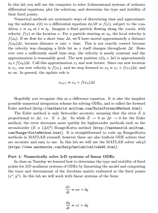
In this lab you will use the computer to solve 2-dimensional systems of ordinary differential equations, plot the solutions, and determine the type and stability of their fixed points. Numerical methods are systematic ways of discretizing time and approximat- ing the solution (t) to a differential equation dr/dt-f(x), subject to the con- dition z = zo at t-to. Imagine a fluid particle flowing along the z-axis, with velocity f(z) at the location r. For a particle starting at zo, the local velocity is f(zo). If we flow for a short time , we'll have moved approximately a distance f(zo), because distance-rate time. This is not exactly correct because the velocity was changing a little bit as z itself changes throughout At. How- ever over a sufficiently small time step, the velocity is nearly constant and the approximation is reasonably good. The new position r(to+ t) is approximately ro+f(ro)At. Call this approximation 1 and now iterate. Since our new location is 1, our new velocity is f(, and we step forward to r2f(i)At, and so on. In general, the update rule is Hopefully you recognize this as a difference equation. It is also the simplest possible numerical integration scheme for solving ODEs, and is called the forward Euler method (http://mathworld.volfram.com/EulerForwardMethod.html). The Euler method is only first-order accurate, meaning that the error E is proportional to t, ie. E x t. So while E 0 as t 0 for the Euler method, the error decreases more quickly for higher-order methods such as the second-order (E x ()2) Runge-Kutta method (http://mathworld.wolfr com/Runge-KuttaKethod.html). It is straightforward to code up Runge-Kutta methods in MATLAB yourself, however there are also built-in ODE solvers that are accurate and easy to use. In this lab we will use the MATLAB solver ode45 (https://www.mathworks.com/help/matlab/ref/ode45.html) Part 1: Numerically solve 2-D systems of linear ODEs In class on Tuesday we learned how to determine the type and stability of fixed points for 2-D nonlinear systems of ODEs by linearizing the model and computing the trace and determinant of the Jacobian matrix evaluated at the fixed points (x.y). In this lab we will work with linear systems of the form: dr