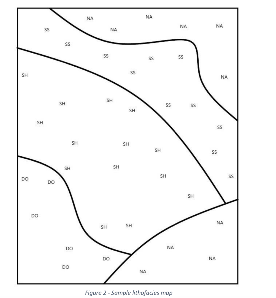
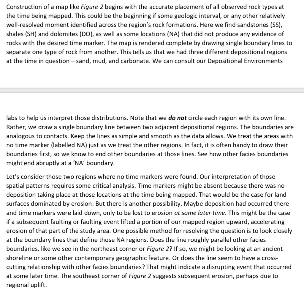
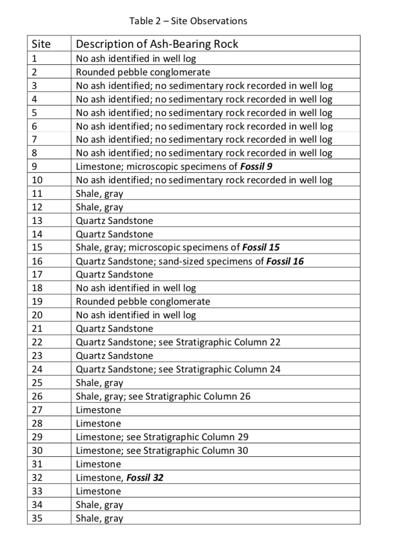
STEP THREE - LITHOFACIES MAPPING We will now place the valley wall outcrops into a larger geologic setting. In this case we can use the blanket of volcanic ash as a time marker that will allow us to pinpoint any rocks in the surrounding area that date to the time of that same volcanic episode. In addition to the valley wall outcrops, we will consider evidence from well borings and a few small roadcuts. In the process, you will produce a lithofacies map. This is a type of map that shows the geographic distribution of formations as if they were captured at a moment in Earth's history. The ash layer will represent that 'moment'. You will map the formations that contain the ash layer. The following figure provides an example of a lithofacies map. Locations are identified by rock type, with facies boundaries drawn to separate those rock types. The boundaries are the equivalent of formation contacts, shown from a map perspective. Because we often associate certain types of sedimentary rocks with unique depositional settings, we can begin to infer the geographic environment at some moment in time. NA NA NA NA SS NA SS SS SS SS SS SH NA SH SH SS SS SH SH SS SH SH SH SS SH SH SH SS DO DO SH DO NA SH SH DO NA DO NA DO NA Figure 2 - Sample lithofacies map Construction of a map like Figure 2 begins with the accurate placement of all observed rock types at the time being mapped. This could be the beginning if some geologic interval, or any other relatively well-resolved moment identified across the region's rock formations. Here we find sandstones (SS), shales (SH) and dolomites (DO), as well as some locations (NA) that did not produce any evidence of rocks with the desired time marker. The map is rendered complete by drawing single boundary lines to separate one type of rock from another. This tells us that we had three different depositional regions at the time in question - sand, mud, and carbonate. We can consult our Depositional Environments labs to help us interpret those distributions. Note that we do not circle each region with its own line. Rather, we draw a single boundary line between two adjacent depositional regions. The boundaries are analogous to contacts. Keep the lines as simple and smooth as the data allows. We treat the areas with no time marker (labelled NA) just as we treat the other regions. In fact, it is often handy to draw their boundaries first, so we know to end other boundaries at those lines. See how other facies boundaries might end abruptly at a 'NA' boundary. Let's consider those two regions where no time markers were found. Our interpretation of those spatial patterns requires some critical analysis. Time markers might be absent because there was no deposition taking place at those locations at the time being mapped. That would be the case for land surfaces dominated by erosion. But there is another possibility. Maybe deposition had occurred there and time markers were laid down, only to be lost to erosion at some later time. This might be the case if a subsequent faulting or faulting event lifted a portion of our mapped region upward, accelerating erosion of that part of the study area. One possible method for resolving the question is to look closely at the boundary lines that define those NA regions. Does the line roughly parallel other facies boundaries, like we see in the northeast corner or Figure 2? If so, we might be looking at an ancient shoreline or some other contemporary geographic feature. Or does the line seem to have a cross- cutting relationship with other facies boundaries? That might indicate a disrupting event that occurred at some later time. The southeast corner of Figure 2 suggests subsequent erosion, perhaps due to regional uplift. Figure 3 - Map of the Study Area 2x 3 X 5X 1X 6X FOOT WALL HANGING WALL Figure 3 is as map of our study area. The five columns in Figure 1 can be found, by reference numbers, lying along a roughly straight line. Other numbered locations locate many additional, contemporary observation sites. The key at the bottom of the map identifies different locations by how observations were made. A larger version of this map also appears on your worksheet. 18 X 13 X 7 X 20% 19X 10 X 14 X 12 x 17X 21 X 11X 16X 15 V 9X 27 X 25 X Table 2 provides details of the observations made at all 35 located sites, specifically the rock type observed to contain the ash layer at each location. Some site descriptions also include mention of fossils or sedimentary structures found in close association with the ash layer. 22 240 28X 23 X 260 290 300 34 X 35X 32V 31 X 33 X Problem 7 -Transfer the relevant rock type information from Table 2 to the draft copy of the Figure 3 map on your worksheet. Draw the lithofacies boundary on the draft map. Then copy the lines only onto a clean version of the map. (4 points) Data sources: * Well log Valley wall exposure Road cut Table 2 - Site Observations Site 6 7 8 9 10 11 12 13 14 15 16 17 Description of Ash-Bearing Rock No ash identified in well log Rounded pebble conglomerate No ash identified; no sedimentary rock recorded in well log No ash identified; no sedimentary rock recorded in well log No ash identified; no sedimentary rock recorded in well log No ash identified; no sedimentary rock recorded in well log No ash identified; no sedimentary rock recorded in well log No ash identified; no sedimentary rock recorded in well log Limestone; microscopic specimens of Fossil 9 No ash identified; no sedimentary rock recorded in well log Shale, gray Shale, gray Quartz Sandstone Quartz Sandstone Shale, gray; microscopic specimens of Fossil 15 Quartz Sandstone; sand-sized specimens of Fossil 16 Quartz Sandstone No ash identified in well log Rounded pebble conglomerate No ash identified in well log Quartz Sandstone Quartz Sandstone; see Stratigraphic Column 22 Quartz Sandstone Quartz Sandstone; see Stratigraphic Column 24 Shale, gray Shale, gray; see Stratigraphic Column 26 Limestone Limestone Limestone; see Stratigraphic Column 29 Limestone; see Stratigraphic Column 30 Limestone Limestone, Fossil 32 Limestone Shale, gray 18 19 20 21 22 23 24 25 26 27 28 29 30 31 32 33 34 35 Shale, gray STEP THREE - LITHOFACIES MAPPING We will now place the valley wall outcrops into a larger geologic setting. In this case we can use the blanket of volcanic ash as a time marker that will allow us to pinpoint any rocks in the surrounding area that date to the time of that same volcanic episode. In addition to the valley wall outcrops, we will consider evidence from well borings and a few small roadcuts. In the process, you will produce a lithofacies map. This is a type of map that shows the geographic distribution of formations as if they were captured at a moment in Earth's history. The ash layer will represent that 'moment'. You will map the formations that contain the ash layer. The following figure provides an example of a lithofacies map. Locations are identified by rock type, with facies boundaries drawn to separate those rock types. The boundaries are the equivalent of formation contacts, shown from a map perspective. Because we often associate certain types of sedimentary rocks with unique depositional settings, we can begin to infer the geographic environment at some moment in time. NA NA NA NA SS NA SS SS SS SS SS SH NA SH SH SS SS SH SH SS SH SH SH SS SH SH SH SS DO DO SH DO NA SH SH DO NA DO NA DO NA Figure 2 - Sample lithofacies map Construction of a map like Figure 2 begins with the accurate placement of all observed rock types at the time being mapped. This could be the beginning if some geologic interval, or any other relatively well-resolved moment identified across the region's rock formations. Here we find sandstones (SS), shales (SH) and dolomites (DO), as well as some locations (NA) that did not produce any evidence of rocks with the desired time marker. The map is rendered complete by drawing single boundary lines to separate one type of rock from another. This tells us that we had three different depositional regions at the time in question - sand, mud, and carbonate. We can consult our Depositional Environments labs to help us interpret those distributions. Note that we do not circle each region with its own line. Rather, we draw a single boundary line between two adjacent depositional regions. The boundaries are analogous to contacts. Keep the lines as simple and smooth as the data allows. We treat the areas with no time marker (labelled NA) just as we treat the other regions. In fact, it is often handy to draw their boundaries first, so we know to end other boundaries at those lines. See how other facies boundaries might end abruptly at a 'NA' boundary. Let's consider those two regions where no time markers were found. Our interpretation of those spatial patterns requires some critical analysis. Time markers might be absent because there was no deposition taking place at those locations at the time being mapped. That would be the case for land surfaces dominated by erosion. But there is another possibility. Maybe deposition had occurred there and time markers were laid down, only to be lost to erosion at some later time. This might be the case if a subsequent faulting or faulting event lifted a portion of our mapped region upward, accelerating erosion of that part of the study area. One possible method for resolving the question is to look closely at the boundary lines that define those NA regions. Does the line roughly parallel other facies boundaries, like we see in the northeast corner or Figure 2? If so, we might be looking at an ancient shoreline or some other contemporary geographic feature. Or does the line seem to have a cross- cutting relationship with other facies boundaries? That might indicate a disrupting event that occurred at some later time. The southeast corner of Figure 2 suggests subsequent erosion, perhaps due to regional uplift. Figure 3 - Map of the Study Area 2x 3 X 5X 1X 6X FOOT WALL HANGING WALL Figure 3 is as map of our study area. The five columns in Figure 1 can be found, by reference numbers, lying along a roughly straight line. Other numbered locations locate many additional, contemporary observation sites. The key at the bottom of the map identifies different locations by how observations were made. A larger version of this map also appears on your worksheet. 18 X 13 X 7 X 20% 19X 10 X 14 X 12 x 17X 21 X 11X 16X 15 V 9X 27 X 25 X Table 2 provides details of the observations made at all 35 located sites, specifically the rock type observed to contain the ash layer at each location. Some site descriptions also include mention of fossils or sedimentary structures found in close association with the ash layer. 22 240 28X 23 X 260 290 300 34 X 35X 32V 31 X 33 X Problem 7 -Transfer the relevant rock type information from Table 2 to the draft copy of the Figure 3 map on your worksheet. Draw the lithofacies boundary on the draft map. Then copy the lines only onto a clean version of the map. (4 points) Data sources: * Well log Valley wall exposure Road cut Table 2 - Site Observations Site 6 7 8 9 10 11 12 13 14 15 16 17 Description of Ash-Bearing Rock No ash identified in well log Rounded pebble conglomerate No ash identified; no sedimentary rock recorded in well log No ash identified; no sedimentary rock recorded in well log No ash identified; no sedimentary rock recorded in well log No ash identified; no sedimentary rock recorded in well log No ash identified; no sedimentary rock recorded in well log No ash identified; no sedimentary rock recorded in well log Limestone; microscopic specimens of Fossil 9 No ash identified; no sedimentary rock recorded in well log Shale, gray Shale, gray Quartz Sandstone Quartz Sandstone Shale, gray; microscopic specimens of Fossil 15 Quartz Sandstone; sand-sized specimens of Fossil 16 Quartz Sandstone No ash identified in well log Rounded pebble conglomerate No ash identified in well log Quartz Sandstone Quartz Sandstone; see Stratigraphic Column 22 Quartz Sandstone Quartz Sandstone; see Stratigraphic Column 24 Shale, gray Shale, gray; see Stratigraphic Column 26 Limestone Limestone Limestone; see Stratigraphic Column 29 Limestone; see Stratigraphic Column 30 Limestone Limestone, Fossil 32 Limestone Shale, gray 18 19 20 21 22 23 24 25 26 27 28 29 30 31 32 33 34 35 Shale, gray