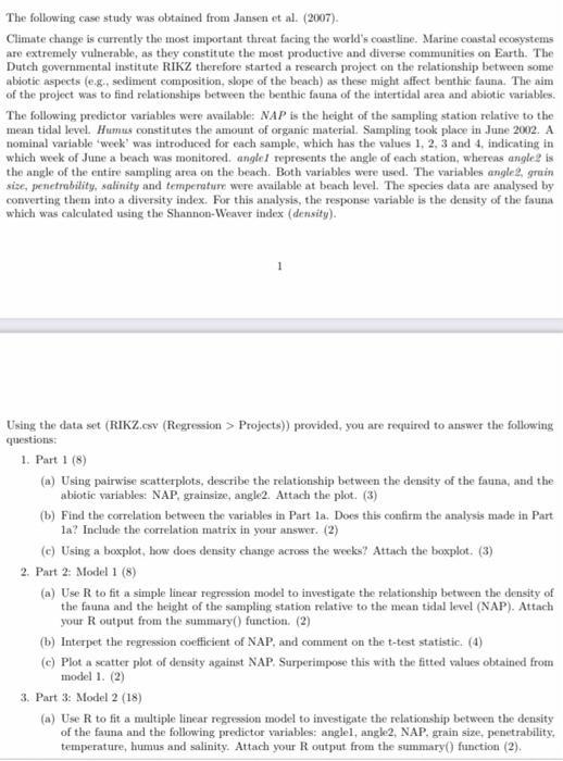
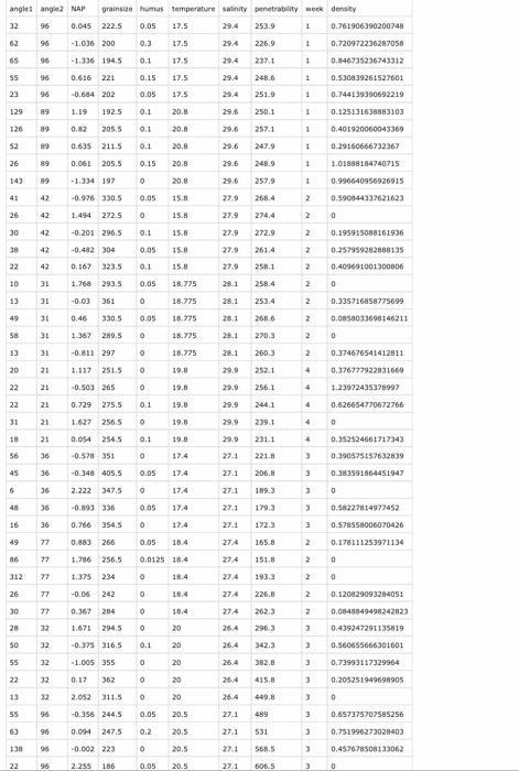
The following case study was obtained from Jansen et al. (2007). Climate change is currently the most important threat facing the world's coastline. Marine coastal ecosystems are extremely vulnerable, as they constitute the most productive and diverse communities on Earth. The Dutch governmental institute RIKZ therefore started a research project on the relationship between some abiotic aspects (e.g., sediment composition, slope of the beach) as these might affect benthic fauna. The aim of the project was to find relationships between the benthic fauna of the intertidal area and abiotice variables. The following predictor variables were available: NAP is the height of the sampling station relative to the mean tidal level. Humus constitutes the amount of organic material. Sampling took place in June 2002. A nominal variable 'week' was introduced for each sample, which has the values 1, 2, 3 and 4, indicating in which week of June a beach was monitored. anglel represents the angle of each station, whereas angle2 is the angle of the entire sampling area on the beach. Both variables were used. The variables angle2, gruin size, penetrability, salinity and temperature were available at beach level. The species data are analysed by converting them into a diversity index. For this analysis, the response variable is the density of the fauna which was calculated using the Shannon-Weaver index (density). 1 Using the data set (RIKZ.csv (Regression > Projects)) provided, you are required to answer the following questions: 1. Part 1 (8) (a) Using pairwise scatterplots, describe the relationship between the density of the fauna, and the abiotic variables: NAP, grainsize, angle2. Attach the plot. (3) (b) Find the correlation between the variables in Part la. Does this confirm the analysis made in Part la? Include the correlation matrix in your answer. (2) (c) Using a boxplot, how does density change across the weeks? Attach the boxplot. (3) 2. Part 2: Model 1 (8) (a) Use R to fit a simple linear regression model to investigate the relationship between the density of the fauna and the height of the sampling station relative to the mean tidal level (NAP). Attach your R output from the summary() function. (2) (b) Interpet the regression coefficient of NAP, and comment on the t-test statistic. (4) (c) Plot a scatter plot of density against NAP. Surperimpose this with the fitted values obtained from model 1. (2) 3. Part 3: Model 2 (18) (a) Use R to fit a multiple linear regression model to investigate the relationship between the density of the fauna and the following predictor variables: anglel, angle2, NAP. grain size, penetrability, temperature, humus and salinity. Attach your R output from the summary() function (2). anglet angle2 NAP grainsize humus temperature salinity penetrability week density 32 96 0.045 222.5 0.05 17.5 29.4 253.9 1. 0.761906390200748 62 96 -1.036 200 0.3 17.5 294 226.9 0.720972236287058 65 96 -1.336 194.5 0.1 17.5 29.4 237.1 1. 0.846715236743312 55 96 0.616 221 0.15 17.5 29.4 248.6 1. 0.530839261527601 23 96 0.684 202 0.05 17.5 29.4 251.9 0.744139390692219 129 89 1.19 192.5 0.1 20.8 29.6 250.1 0.125131638883103 126 89 0.82 205.5 0.1 20.8 29.6 257.1 0.401920060043369 52 89 0.635 211.5 0.1 20.8 29.6 247.9 0.29160666732367 26 89 0.061 205.5 0.15 20.8 29.6 248.9 1.01888184740715 143 89 -1.334 197 20.8 29.6 257.9 0.996640956926915 42 -0.976 330.5 0.05 268.4 41 15.8 27.9 0.590844332621623 26 42 1.494 272.5 15.8 27.9 274.4 30 42 -0.201 296.5 0.1 15.8 27.9 272.9 0.195915088161936 38 42 --0.482 304 0.05 15.8 27.9 261.4 0.257959282888135 22 42 0.167 323.5 0.1 15.8 27.9 258.1 0.409691001300o806 10 31 1.768 293.5 0.05 18.775 28.1 258.4 13 31 -0.03 361 18.775 28.1 253.4 0.335716858775699 49 31 0.46 330.5 0.05 18.775 28.1 268.6 0.0858033698146211 58 31 1.367 289.5 18.775 28.1 270.3 13 31 -0.811 297 18.775 28.1 260.3 2. 0.374676541412811 20 21 1.117 251.5 19. 29.9 252.1 4. 0.376777922031669 22 21 -0.503 265 19.8 29.9 256.1 4. 1.23972435378997 22 21 0.729 275.5 0.1 19.8 29.9 244.1 4 0.626654770672766 31 21 1.627 256.5 19.8 29.9 239.1 18 24 0.054 254.5 0.1 19.8 29.9 231.1 0.352524661717343 56 36 -0.578 351 17.4 27.1 221.8 0.390575157632839 45 36 -0.348 405.5 0.05 17.4 27.1 206.8 0.383591864451947 36 2.222 347.5 17.4 27.1 189.3 48 36 -0.893 336 0.05 17.4 27.1 179.3 0.58227814977452 16 36 0.766 354.5 17.4 27.4 172.3 0.5785s8006070426 49 77 0.883 266 0.05 18.4 274 165.8 2 0.178111253971134 86 1.786 256.5 0.0125 16.4 274 151.8 312 77 1.375 234 18.4 27.4 193.3 26 77 -0.06 242 18.4 27.4 226.8 0.120829093284051 30 77 0.367 284 18.4 274 262.3 0.0848849498242823 28 32 1.671 294.5 20 26.4 296.3 0.439247291135819 50 32 -0.375 316.5 0.1 20 26.4 342.3 3. 0.560655666301601 5 32 1.005 355 20 26.4 382.8 0.73993117329964 22 32 0.17 362 20 26.4 415.8 0.205251949698905 13 32 2.052 311.5 20 26.4 449.8 55 96 0.356 244.5 0.05 20.5 27.1 489 3. 0.657375707585256 63 96 0.094 247,5 0.2 20.5 27.1 531 0.751996273028403 138 96 -0.002 223 20.5 27.1 568.5 0.45767850813062 22 96 2.255 186 0.05 20.5 27.1 606.5 3 o o o o