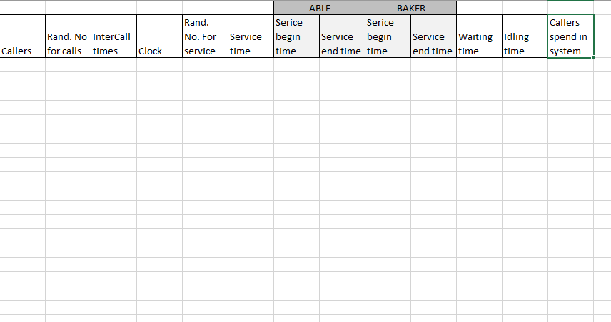
This is the starting point the table should be completed .

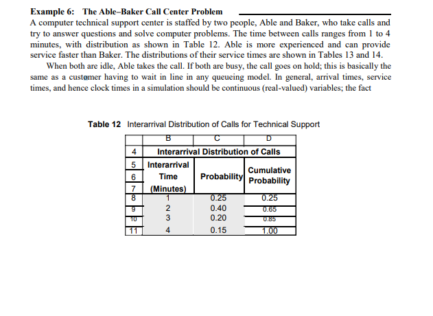
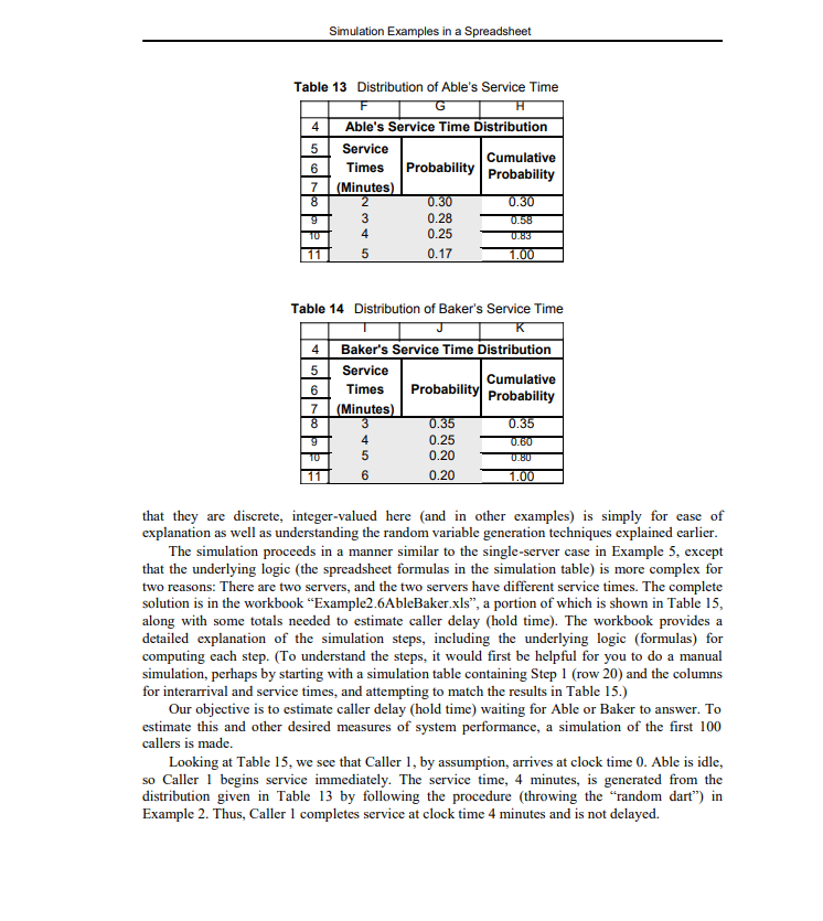
Example 6: The Able-Baker Call Center Problem A computer technical support center is staffed by two people, Able and Baker, who take calls and try to answer questions and solve computer problems. The time between calls ranges from 1 to 4 minutes, with distribution as shown in Table 12. Able is more experienced and can provide service faster than Baker. The distributions of their service times are shown in Tables 13 and 14. When both are idle, Able takes the call. If both are busy, the call goes on hold; this is basically the same as a customer having to wait in line in any queueing model. In general, arrival times, service times, and hence clock times in a simulation should be continuous (real-valued) variables; the fact Table 12 Interarrival Distribution of Calls for Technical Support B 4 Interarrival Distribution of Calls 5 Interarrival Cumulative Time Probability Probability 7 (Minutes) 8 1 0.25 0.25 9 2 0.40 0.65 TU 3 0.20 11 4 0.15 1.00 6 0.85 Simulation Examples in a Spreadsheet Table 13 Distribution of Able's Service Time G 4 Able's Service Time Distribution 5 Service Cumulative 6 Times Probability Probability 7 (Minutes) 8 2 0.30 0.30 0.28 0.58 4 0.25 11 5 0.17 1.00 TU 0.85 6 Table 14 Distribution of Baker's Service Time 4 Baker's Service Time Distribution 5 Service Cumulative 6 Times Probability Probability 7 (Minutes) 8 3 0.35 0.35 4 0.25 0.60 TU 5 0.20 11 6 0.20 1.00 0.80 that they are discrete, integer-valued here (and in other examples) is simply for ease of explanation as well as understanding the random variable generation techniques explained earlier. The simulation proceeds in a manner similar to the single-server case in Example 5, except that the underlying logic (the spreadsheet formulas in the simulation table) is more complex for two reasons: There are two servers, and the two servers have different service times. The complete solution is in the workbook Example2.6AbleBaker.xls, a portion of which is shown in Table 15, along with some totals needed to estimate caller delay (hold time). The workbook provides a detailed explanation of the simulation steps, including the underlying logic (formulas) for computing each step. (To understand the steps, it would first be helpful for you to do a manual simulation, perhaps by starting with a simulation table containing Step 1 (row 20) and the columns for interarrival and service times, and attempting to match the results in Table 15.) Our objective is to estimate caller delay (hold time) waiting for Able or Baker to answer. To estimate this and other desired measures of system performance, a simulation of the first 100 callers is made. Looking at Table 15, we see that Caller 1, by assumption, arrives at clock time 0. Able is idle, so Caller 1 begins service immediately. The service time, 4 minutes, is generated from the distribution given in Table 13 by following the procedure (throwing the random dart) in Example 2. Thus, Caller I completes service at clock time 4 minutes and is not delayed. Rand. No. For service Rand. No InterCall for calls times ABLE BAKER Serice Service begin Service Waiting Idling end time time end time time time Serice begin time Service time Callers spend in system Callers Clock