A Course In Mathematical Methods For Physicists 1st Edition Russell L Herman - Solutions

Find all \(z\) such that \(\cos z=2\), or explain why there are none. You will need to consider \(\cos (x+i y)\) and equate real and imaginary parts of the resulting expression similar to Problem 5.Data from Problem 5Show that \(\sin (x+i y)=\sin x \cosh y+i \cos x \sinh y\) using trigonometric
Find the principal value of \(i^{i}\). Rewrite the base, \(i\), as an exponential first.
Consider the circle \(|z-1|=1\).a. Rewrite the equation in rectangular coordinates by setting \(z=\) \(x+i y\).b. Sketch the resulting circle using part a.c. Consider the image of the circle under the mapping \(f(z)=z^{2}\), given by \(\left|z^{2}-1\right|=1\).i. By inserting \(z=r e^{i
Find the real and imaginary parts of the functions:a. \(f(z)=z^{3}\).b. \(f(z)=\sinh (z)\).c. \(f(z)=\cos \bar{z}\).
Find the derivative of each function in Problem 9 when the derivative exists. Otherwise, show that the derivative does not exist.Data from Problem 9Find the real and imaginary parts of the functions:
Let \(f(z)=u+i v\) be differentiable. Consider the vector field given by \(\mathbf{F}=v \mathbf{i}+u \mathbf{j}\). Show that the equations \(abla \cdot \mathbf{F}=\mathbf{0}\) and \(abla \times \mathbf{F}=\mathbf{0}\) are equivalent to the Cauchy-Riemann Equations. [You will need to recall from
What parametric curve is described by the function\[\gamma(t)=(t-3)+i(2 t+1)\]\(0 \leq t \leq 2\) ? [What would you do if you were instead considering the parametric equations \(x=t-3\) and \(y=2 t+1]\)
Write the equation that describes the circle of radius 3 that is centered at \(z=2-i\) in (a) Cartesian form (in terms of \(x\) and \(y\) ); (b) polar form (in terms of \(\theta\) and \(r\) ); (c) complex form (in terms of \(z, r\), and \(e^{i \theta}\) ).
Consider the function \(u(x, y)=x^{3}-3 x y^{2}\).a. Show that \(u(x, y)\) is harmonic; that is, \(abla^{2} u=0\).b. Find its harmonic conjugate, \(v(x, y)\).c. Find a differentiable function, \(f(z)\), for which \(u(x, y)\) is the real part.d. Determine \(f^{\prime}(z)\) for the function in partc.
Evaluate the following integrals:a. \(\int_{C} \bar{z} d z\), where \(C\) is the parabola \(y=x^{2}\) from \(z=0\) to \(z=1+i\).b. \(\int_{C} f(z) d z\), where \(f(z)=2 z-\bar{z}\) and \(C\) is the path from \(z=0\) to \(z=2+i\) consisting of two line segments from \(z=0\) to \(z=2\) and then
Let \(C\) be the positively oriented ellipse \(3 x^{2}+y^{2}=9\). Define\[F\left(z_{0}\right)=\int_{C} \frac{z^{2}+2 z}{z-z_{0}} d z\]Find \(F(2 i)\) and \(F(2)\). [Sketch the ellipse in the complex plane. Use the Cauchy Integral Theorem with an appropriate \(f(z)\), or Cauchy's Theorem if
Show that\[\int_{C} \frac{d z}{(z-1-i)^{n+1}}=\left\{\begin{array}{cc} 0, & n eq 0 \\ 2 \pi i, & n=0 \end{array}\right.\]for \(C\) the boundary of the square \(0 \leq x \leq 2,0 \leq y \leq 2\) taken counterclockwise. [Use the fact that contours can be deformed into simpler shapes (like a
Show that for \(g\) and \(h\) analytic functions at \(z_{0}\), with \(g\left(z_{0}\right) eq 0, h\left(z_{0}\right)=0\), and \(h^{\prime}\left(z_{0}\right) eq 0\),\[\operatorname{Res}\left[\frac{g(z)}{h(z)} ; z_{0}\right]=\frac{g\left(z_{0}\right)}{h^{\prime}\left(z_{0}\right)}\]
For the following, determine if the given point is a removable singularity, an essential singularity, or a pole (indicate its order).a. \(\frac{1-\cos z}{z^{2}}, \quad z=0\).b. \(\frac{\sin z}{z^{2}}, \quad z=0\).c. \(\frac{z^{2}-1}{(z-1)^{2}}, \quad z=1\)d. \(z e^{1 / z}, \quad z=0\).e. \(\cos
Find the Laurent series expansion for \(f(z)=\frac{\sinh z}{z^{3}}\) about \(z=0\). [You need to first do a MacLaurin series expansion for the hyperbolic sine.]
Find series representations for all indicated regions.a. \(f(z)=\frac{z}{z-1},|z|1\).b. \(f(z)=\frac{1}{(z-i)(z+2)},|z|
Find the residues at the given points:a. \(\frac{2 z^{2}+3 z}{z-1}\) at \(z=1\).b. \(\frac{\ln (1+2 z)}{z}\) at \(z=0\).c. \(\frac{\cos z}{(2 z-\pi)^{3}}\) at \(z=\frac{\pi}{2}\).
Consider the integral \(\int_{0}^{2 \pi} \frac{d \theta}{5-4 \cos \theta}\).a. Evaluate this integral by making the substitution \(2 \cos \theta=z+\frac{1}{z}\), \(z=e^{i \theta}\), and using complex integration methods.b. In the 1800 , Weierstrass introduced a method for computing integrals
Do the following integrals:a. \(\oint_{|z-i|=3} \frac{e^{z}}{z^{2}+\pi^{2}} d z\)b. \(\oint_{|z-i|=3} \frac{z^{2}-3 z+4}{z^{2}-4 z+3} d z\).c. \(\int_{-\infty}^{\infty} \frac{\sin x}{x^{2}+4} d x\). [This is \(\operatorname{Im} \int_{-\infty}^{\infty} \frac{e^{i x}}{x^{2}+4} d x\).]
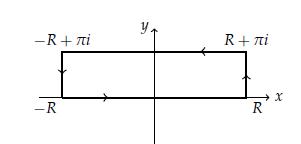
Evaluate the integral \(\int_{0}^{\infty} \frac{(\ln x)^{2}}{1+x^{2}} d x\).[Replace \(x\) with \(z=e^{t}\) and use the rectangular contour in Figure 7. 55 with \(R \rightarrow \infty\).]Data from Figure 7.55 -R+i R+i -R R X
Do the following integrals for fun!a. For \(C\) the boundary of the square \(|x| \leq 2,|y| \leq 2\),\[\oint_{C} \frac{d z}{z(z-1)(z-3)^{2}}\]b.\[\int_{0}^{\pi} \frac{\sin ^{2} \theta}{13-12 \cos \theta} d \theta\]c.\[\int_{-\infty}^{\infty} \frac{d x}{x^{2}+5 x+6}\]d.\[\int_{0}^{\infty} \frac{\cos
Consider the set of vectors \((-1,1,1),(1,-1,1),(1,1,-1)\).a. Use the Gram-Schmidt process to find an orthonormal basis for \(R^{3}\) using this set in the given order.b. What do you get if you do reverse the order of these vectors?
Use the Gram-Schmidt process to find the first four orthogonal polynomials satisfying the following:a. Interval: \((-\infty, \infty)\) Weight Function: \(e^{-x^{2}}\).b. Interval: \((0, \infty)\) Weight Function: \(e^{-x}\).
Find \(P_{4}(x)\) usinga. The Rodrigues Formula in Equation (6.20).b. The three-term recursion formula in Equation (6.22).Data from 6.20 Data from 6.22 Pn(x) 1 dn 2"n! drn (1)", n No.
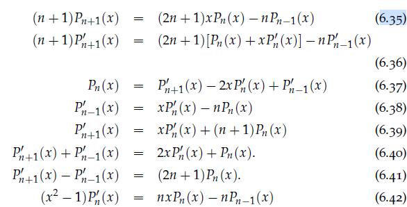
In Equations (6.35) through (6.42), we provide several identities for Legendre polynomials. Derive the results in Equations (6.36) through (6.42) as described in the text. Namely,a. Differentiating Equation (6.35) with respect to \(x\), derive Equation \((6.36)\).b. Derive Equation (6.37) by
Use the recursion relation (6.22) to evaluate \(\int_{-1}^{1} x P_{n}(x) P_{m}(x) d x, n \leq\) \(m\).Data from 6.22 (n+1)Pn+1(x) = (2n+1)xPn(x) - nPn-1(x), n = 1,2,....
Expand the following in a Fourier-Legendre series for \(x \in(-1,1)\).a. \(f(x)=x^{2}\).b. \(f(x)=5 x^{4}+2 x^{3}-x+3\).c. \(f(x)=\left\{\begin{array}{cc}-1, & -1
Use integration by parts to show \(\Gamma(x+1)=x \Gamma(x)\).
Prove the double factorial identities:\[(2 n)!!=2^{n} n!\]and\[(2 n-1)!!=\frac{(2 n)!}{2^{n} n!}\]
Express the following as Gamma functions. Namely, noting the form \(\Gamma(x+1)=\int_{0}^{\infty} t^{x} e^{-t} d t\) and using an appropriate substitution, each expression can be written in terms of a Gamma function.a. \(\int_{0}^{\infty} x^{2 / 3} e^{-x} d x\).b. \(\int_{0}^{\infty} x^{5}
The coefficients \(C_{k}^{p}\) in the binomial expansion for \((1+x)^{p}\) are given by\[C_{k}^{p}=\frac{p(p-1) \cdots(p-k+1)}{k!}\]a. Write \(C_{k}^{p}\) in terms of Gamma functions.b. For \(p=1 / 2\), use the properties of Gamma functions to write \(C_{k}^{1 / 2}\) in terms of factorials.c.
The Hermite polynomials, \(H_{n}(x)\), satisfy the following:i. \(=\int_{-\infty}^{\infty} e^{-x^{2}} H_{n}(x) H_{m}(x) d x=\sqrt{\pi} 2^{n} n!\delta_{n, m}\).ii. \(H_{n}^{\prime}(x)=2 n H_{n-1}(x)\).iii. \(H_{n+1}(x)=2 x H_{n}(x)-2 n H_{n-1}(x)\).iv. \(H_{n}(x)=(-1)^{n} e^{x^{2}} \frac{d^{n}}{d
In Maple, one can type simplify(LegendreP(2*n-2,0)-LegendreP(2* \(\mathbf{n}, \mathbf{0})\) ); to find a value for \(P_{2 n-2}(0)-P_{2 n}(0)\). It gives the result in terms of Gamma functions. However, in Example 6. 10 for Fourier-Legendre series, the value is given in terms of double factorials!
A solution of Bessel's equation, \(x^{2} y^{\prime \prime}+x y^{\prime}+\left(x^{2}-n^{2}\right) y=0\), can be found using the guess \(y(x)=\sum_{j=0}^{\infty} a_{j} x^{j+n}\). One obtains the recurrence relation \(a_{j}=\frac{-1}{j(2 n+j)} a_{j-2}\). Show that for
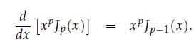
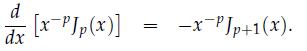
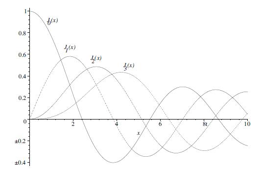
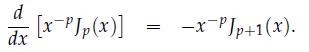
Use the infinite series in the Problem 13 derive the derivative identities \((6.59)\) and \((6.60)\) :a. \(\frac{d}{d x}\left[x^{n} J_{n}(x)\right]=x^{n} J_{n-1}(x)\).b. \(\frac{d}{d x}\left[x^{-n} J_{n}(x)\right]=-x^{-n} J_{n+1}(x)\).Data from Problem 13A solution of Bessel's equation, \(x^{2}
Prove the following identities based on those in the Problem 14:a. \(J_{p-1}(x)+J_{p+1}(x)=\frac{2 p}{x} J_{p}(x)\).b. \(J_{p-1}(x)-J_{p+1}(x)=2 J_{p}^{\prime}(x)\).Data from Problem 14Use the infinite series in the Problem 13 derive the derivative identities \((6.59)\) and \((6.60)\).
Use the derivative identities of Bessel functions,(6.59)-(6.60), and integration by parts to show that\[\int x^{3} J_{0}(x) d x=x^{3} J_{1}(x)-2 x^{2} J_{2}(x)+C\]Data from 6.59Data from 6.60 d [x Jp(x)] dx xJp-1(x).
Use the generating function to find \(J_{n}(0)\) and \(J_{n}^{\prime}(0)\).
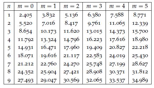
Bessel functions \(J_{p}(\lambda x)\) are solutions of \(x^{2} y^{\prime \prime}+x y^{\prime}+\left(\lambda^{2} x^{2}-p^{2}\right) y=\) 0 . Assume that \(x \in(0,1)\) and that \(J_{p}(\lambda)=0\) and \(J_{p}(0)\) is finite.a. Show that this equation can be written in the form \[\frac{d}{d
We can rewrite Bessel functions, \(J_{v}(x)\), in a form that will allow the order to be non-integer by using the gamma function. You will need the results from Problem \(12 b\) for \(\Gamma\left(k+\frac{1}{2}\right)\).a. Extend the series definition of the Bessel function of the first kind of
In this problem you will derive the expansion\[x^{2}=\frac{c^{2}}{2}+4 \sum_{j=2}^{\infty} \frac{J_{0}\left(\alpha_{j} x\right)}{\alpha_{j}^{2} J_{0}\left(\alpha_{j} c\right)}, \quad 0where the \(\alpha_{j}{ }^{\prime} s\) are the positive roots of \(J_{1}(\alpha c)=0\), by following the below
Prove that if \(u(x)\) and \(v(x)\) satisfy the general homogeneous boundary conditions\[\begin{array}{r} \alpha_{1} u(a)+\beta_{1} u^{\prime}(a)=0 \\ \alpha_{2} u(b)+\beta_{2} u^{\prime}(b)=0 \tag{6.173} \end{array}\]at \(x=a\) and \(x=b\), then\[p(x)\left[u(x) v^{\prime}(x)-v(x)
Prove Green's identity \(\int_{a}^{b}(u \mathcal{L} v-v \mathcal{L} u) d x=\left.\left[p\left(u v^{\prime}-v u^{\prime}\right)\right]\right|_{a} ^{b}\) for the general Sturm-Liouville operator \(\mathcal{L}\).
Find the adjoint operator and its domain for \(L u=u^{\prime \prime}+4 u^{\prime}-3 u\), \(u^{\prime}(0)+4 u(0)=0, u^{\prime}(1)+4 u(1)=0\).
Show that a Sturm-Liouville operator with periodic boundary conditions on \([a, b]\) is self-adjoint if and only if \(p(a)=p(b)\). [Recall that periodic boundary conditions are given as \(u(a)=u(b)\) and \(u^{\prime}(a)=u^{\prime}(b)\).]
The Hermite differential equation is given by \(y^{\prime \prime}-2 x y^{\prime}+\lambda y=0\). Rewrite this equation in self-adjoint form. From the Sturm-Liouville form obtained, verify that the differential operator is self adjoint on \((-\infty, \infty)\). Give the integral form for the
Find the eigenvalues and eigenfunctions of the given Sturm-Liouville problems:a. \(y^{\prime \prime}+\lambda y=0, y^{\prime}(0)=0=y^{\prime}(\pi)\).b. \(\left(x y^{\prime}\right)^{\prime}+\frac{\lambda}{x} y=0, y(1)=y\left(e^{2}\right)=0\).
The eigenvalue problem \(x^{2} y^{\prime \prime}-\lambda x y^{\prime}+\lambda y=0\) with \(y(1)=y(2)=0\) is not a Sturm-Liouville eigenvalue problem. Show that none of the eigenvalues are real by solving this eigenvalue problem.
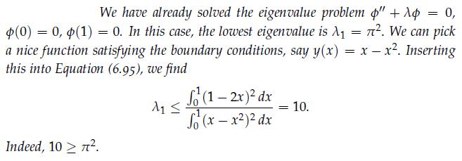
In Example 6. 20, we found a bound on the lowest eigenvalue for the given eigenvalue problem.a. Verify the computation in the example.b. Apply the method using\[y(x)=\left\{\begin{array}{cc} x, & 0.\]Is this an upper bound on \(\lambda_{1}\) ?c. Use the Rayleigh quotient to obtain a good upper
Use the method of eigenfunction expansions to solve the problems:a. \(y^{\prime \prime}+4 y=x^{2}, \quad y^{\prime}(0)=y^{\prime}(1)=0\).b. \(y+4 y=x^{2} \quad y(0)=y(1)=0\).
Determine the solvability conditions for the nonhomogeneous boundary value problem: \(u^{\prime}(\pi / 4)=\beta\).
Consider the problem \(y^{\prime \prime}=\sin x, y^{\prime}(0)=0, y(\pi)=0\).a. Solve by direct integration.b. Determine the Green's function.c. Solve the boundary value problem using the Green's function.d. Change the boundary conditions to \(y^{\prime}(0)=5, y(\pi)=-3\).i. Solve by direct
Consider the problem:\[\frac{\partial^{2} G}{\partial x^{2}}=\delta\left(x-x_{0}\right), \quad \frac{\partial G}{\partial x}\left(0, x_{0}\right)=0, \quad G\left(\pi, x_{0}\right)=0\]a. Solve by direct integration.b. Compare this result to the Green's function in part b of Problem 31.c. Verify that
Consider the boundary value problem: \(y^{\prime \prime}-y=x, x \in(0,1)\), with boundary conditions \(y(0)=y(1)=0\).a. Find a closed form solution without using Green's functions.b. Determine the closed form Green's function using the properties of Green's functions. Use this Green's function to
Solve the following boundary value problems directly, when possible.a. \(\quad x^{\prime \prime}+x=2, \quad x(0)=0, \quad x^{\prime}(1)=0\).b. \(y^{\prime \prime}+2 y^{\prime}-8 y=0, \quad y(0)=1, \quad y(1)=0\).c. \(y^{\prime \prime}+y=0, \quad y(0)=1, \quad y(\pi)=0\).
Find product solutions, \(u(x, t)=b(t) \phi(x)\), to the heat equation satisfying the boundary conditions \(u_{x}(0, t)=0\) and \(u(L, t)=0\). Use these solutions to find a general solution of the heat equation satisfying these boundary conditions.
Find product solutions, \(u(x, t)=b(t) \phi(x)\), to the wave equation satisfying the boundary conditions \(u(0, t)=0\) and \(u_{x}(1, t)=0\). Use these solutions to find a general solution of the heat equation satisfying these boundary conditions.
Consider the following boundary value problems. Determine the eigenvalues \(\lambda\) and eigenfunctions \(y(x)\) for each problem.a. \(y^{\prime \prime}+\lambda y=0, \quad y(0)=0, \quad y^{\prime}(1)=0\).b. \(y^{\prime \prime}-\lambda y=0, \quad y(-\pi)=0, \quad y^{\prime}(\pi)=0\).c. \(x^{2}
Consider the boundary value problem for the deflection of a horizontal beam fixed at one end,\[\frac{d^{4} y}{d x^{4}}=C, \quad y(0)=0, \quad y^{\prime}(0)=0, \quad y^{\prime \prime}(L)=0, \quad y^{\prime \prime \prime}(L)=0\]Solve this problem assuming that \(C\) is a constant.
Write \(y(t)=3 \cos 2 t-4 \sin 2 t\) in the form \(y(t)=A \cos (2 \pi f t+\phi)\).
Derive the coefficients \(b_{n}\) in Equation (5.24).Data from 5.24 an 1-1 2 f(x) cos nx dx, n = 0,1,2,..., 0 2 bn f(x) sin nx dx, n = 1,2,.... IL JO
Let \(f(x)\) be defined for \(x \in[-L, L]\). Parseval's identity is given by\[\frac{1}{L} \int_{-L}^{L} f^{2}(x) d x=\frac{a_{0}^{2}}{2}+\sum_{n=1}^{\infty} a_{n}^{2}+b_{n}^{2}\]Assuming the the Fourier series of \(f(x)\) converges uniformly in \((-L, L)\), prove Parseval's identity by multiplying
Consider the square wave function\[f(x)=\left\{\begin{array}{rc} 1, & 0
For the following sets of functions: (i) show that each is orthogonal on the given interval, and (ii) determine the corresponding orthonormal set. a. \(\{\sin 2 n x\}, \quad n=1,2,3, \ldots, \quad 0 \leq x \leq \pi\).b. \(\{\cos n \pi x\}, \quad n=0,1,2, \ldots, \quad 0 \leq x \leq 2\).c.
Consider \(f(x)=4 \sin ^{3} 2 x\).a. Derive the trigonometric identity giving \(\sin ^{3} \theta\) in terms of \(\sin \theta\) and \(\sin 3 \theta\) using DeMoivre's Formula.b. Find the Fourier series of \(f(x)=4 \sin ^{3} 2 x\) on \([0,2 \pi]\) without computing any integrals.
Find the Fourier series of the following:a. \(f(x)=x, x \in[0,2 \pi]\).b. \(f(x)=\frac{x^{2}}{4},|x|
Find the Fourier series of each function \(f(x)\) of period \(2 \pi\). For each series, plot the Nth partial sum,\[S_{N}=\frac{a_{0}}{2}+\sum_{n=1}^{N}\left[a_{n} \cos n x+b_{n} \sin n x\right]\]for \(N=5,10,50\) and describe the convergence (Is it fast? What is it converging to?, etc.) [Some
Find the Fourier series of \(f(x)=x\) on the given interval. Plot the Nth partial sums and describe what you see.a. \(0
The result in Problem 12b, above gives a Fourier series representation of \(\frac{x^{2}}{4}\). By picking the right value for \(x\) and a little arrangement of the series, show that
Sketch (by hand) the graphs of each of the following functions over four periods. Then sketch the extensions of each of the functions as both an even and odd periodic function. Determine the corresponding Fourier sine and cosine series, and verify the convergence to the desired function using
Consider the function \(f(x)=x,-\pi
Consider the function \(f(x)=x, 0
Differentiate the Fourier sine series term by term in Problem 18. Show that the result is not true. Why not?Data from Problem 18Consider the function \(f(x)=x, 0
Rewrite the solution to Problem 2 and identify the initial value Green's function.Data from Problem 2Find product solutions, \(u(x, t)=b(t) \phi(x)\), to the heat equation satisfying the boundary conditions \(u_{x}(0, t)=0\) and \(u(L, t)=0\). Use these solutions to find a general solution of the
Rewrite the solution to Problem 3 and identify the initial value Green's functions.Data from Problem 3Find product solutions, \(u(x, t)=b(t) \phi(x)\), to the wave equation satisfying the boundary conditions \(u(0, t)=0\) and \(u_{x}(1, t)=0\). Use these solutions to find a general solution of the
Solve the general logistic problem,\[\begin{equation*} \frac{d y}{d t}=k y-c y^{2}, \quad y(0)=y_{0} \tag{4.86} \end{equation*}\]using separation of variables. 0.6 0.4 0.2 0 -0.2 -0.4 Nonlinear Linear -0.6 0 2 4 6 8 10
Find the equilibrium solutions and determine their stability for the following systems. For each case, draw representative solutions and phase lines.a. \(y^{\prime}=y^{2}-6 y-16\).b. \(y^{\prime}=\cos y\).c. \(y^{\prime}=y(y-2)(y+3)\).d. \(y^{\prime}=y^{2}(y+1)(y-4)\).
For \(y^{\prime}=y-y^{2}\), find the general solution corresponding to \(y(0)=y_{0}\). Provide specific solutions for the following initial conditions and sketch them:a. \(y(0)=0.25\),b. \(y(0)=1.5\), andc. \(y(0)=-0.5\).
For each problem, determine equilibrium points, bifurcation points, and construct a bifurcation diagram. Discuss the different behaviors in each system.a. \(y^{\prime}=y-\mu y^{2}\)b. \(y^{\prime}=y(\mu-y)(\mu-2 y)\)c. \(x^{\prime}=\mu-x^{3}\)d. \(x^{\prime}=x-\frac{\mu x}{1+x^{2}}\)
Consider the family of differential equations \(x^{\prime}=x^{3}+\delta x^{2}-\mu x\).a. Sketch a bifurcation diagram in the \(x \mu\)-plane for \(\delta=0\).b. Sketch a bifurcation diagram in the \(x \mu\)-plane for \(\delta>0\).Pick a few values of \(\delta\) and \(\mu\) in order to get a feel
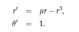
System (4.63) can be solved exactly. Integrate the \(r\)-equation using separation of variables. For initial conditions (a) \(r(0)=0.25, \theta(0)=0\), and (b) \(r(0)=1.5, \theta(0)=0\), and \(\mu=1.0\), find and plot the solutions in the \(x y\)-plane, showing the approach to a limit cycle.Data
Consider the system\[\begin{aligned} x^{\prime} & =-y+x\left[\mu-x^{2}-y^{2}\right] \\ y^{\prime} & =x+y\left[\mu-x^{2}-y^{2}\right] \end{aligned}\]Rewrite this system in polar form. Look at the behavior of the \(r\) equation and construct a bifurcation diagram in \(\mu r\) space. What might
Find the fixed points of the following systems. Linearize the system about each fixed point and determine the nature and stability in the neighborhood of each fixed point, when possible. Verify your findings by plotting phase portraits using a computer.a.\[\begin{aligned} x^{\prime} & =x(100-x-2
Plot phase portraits for the Lienard system\[\begin{aligned} & x^{\prime}=y-\mu\left(x^{3}-x\right) \\ & y^{\prime}=-x \end{aligned}\]for a small and a not so small value of \(\mu\). Describe what happens as one varies \(\mu\).
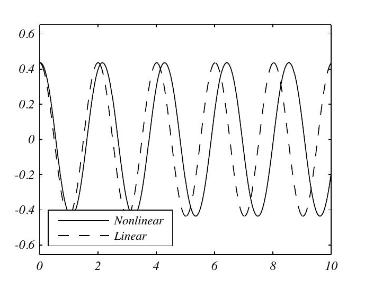
Consider the period of a nonlinear pendulum. Let the length be \(L=1.0\) \(\mathrm{m}\) and \(g=9.8 \mathrm{~m} / \mathrm{s}^{2}\). Sketch \(T\) versus the initial angle \(\theta_{0}\), and compare the linear and nonlinear values for the period. For what angles can you use the linear approximation
Another population model is one in which species compete for resources, such as a limited food supply. Such a model is given by\[\begin{aligned} & x^{\prime}=a x-b x^{2}-c x y \\ & y^{\prime}=d y-e y^{2}-f x y \end{aligned}\]In this case, assume that all constants are positive.a. Describe the
Consider a model of a food chain of three species. Assume that each population on its own can be modeled by logistic growth. Let the species be labeled by \(x(t), y(t)\), and \(z(t)\). Assume that population \(x\) is at the bottom of the chain. That population will be depleted by population \(y\).
Derive the first integral of the Lotka-Volterra system, \(a \ln y+d \ln x-\) \(c x-b y=C\).
Show that the system \(x^{\prime}=x-y-x^{3}, y^{\prime}=x+y-y^{3}\), has at least one limit cycle by picking an appropriate \(\psi(x, y)\) in Dulac's Criteria.
The Lorenz Model is a simple model for atmospheric convection developed by Edward Lorenz in 1963. The system is given by three equations:\[\begin{aligned} \frac{d x}{d t} & =\sigma(y-x) \\ \frac{d y}{d t} & =x(ho-z)-y \\ \frac{d z}{d t} & =x y-\beta z \end{aligned}\]a. Find the equilibrium
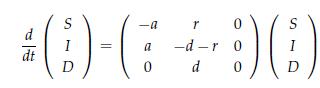
The Michaelis-Menten kinetics reaction is given by\[E+S \underset{k_{1}}{\stackrel{k_{3}}{\longrightarrow}} E S \underset{k_{2}}{\longrightarrow} E+P\]The resulting system of equations for the chemical concentrations is\[\begin{align*} \frac{d[S]}{d t} & =-k_{1}[E][S]+k_{3}[E S] \\ \frac{d[E]}{d
In Equation (3.153), we saw a linear version of an epidemic model. The commonly used nonlinear SIR model is given by\[\begin{align*} \frac{d S}{d t} & =-\beta S I \\ \frac{d I}{d t} & =\beta S I-\gamma I \\ \frac{d R}{d t} & =\gamma I \tag{4.88} \end{align*}\]where \(S\) is the
An undamped, unforced Duffing Equation, \(\ddot{x}+\omega^{2} x+\epsilon x^{3}=0\), can be solved exactly in terms of elliptic functions. Determine the solution of this equation and determine if there are any restrictions on the parameters.
Differentiate the Fourier sine series by term in Problem 18. Show that the result is not the derivative of \(f(x)=x\).Data from Problem 18An undamped, unforced Duffing Equation, \(\ddot{x}+\omega^{2} x+\epsilon x^{3}=0\), can be solved exactly in terms of elliptic functions. Determine the solution
Evaluate the following in terms of elliptic integrals, and compute the values to four decimal places.a. \(\int_{0}^{\pi / 4} \frac{d \theta}{\sqrt{1-\frac{1}{2} \sin ^{2} \theta}}\).b. \(\int_{0}^{\pi / 2} \frac{d \theta}{\sqrt{1-\frac{1}{4} \sin ^{2} \theta}}\).c. \(\int_{0}^{2} \frac{d
Express the vector \(\mathbf{v}=(1,2,3)\) as a linear combination of the vectors \(\mathbf{a}_{1}=(1,1,1), \mathbf{a}_{2}=(1,0,-2)\), and \(\mathbf{a}_{3}=(2,1,0)\).
A symmetric matrix is one for which the transpose of the matrix is the same as the original matrix, \(A^{T}=A\). An antisymmetric matrix is one that satisfies \(A^{T}=-A\).a. Show that the diagonal elements of an \(n \times n\) antisymmetric matrix are all zero.b. Show that a general \(3 \times 3\)
Consider the matrix representations for two-dimensional rotations of vectors by angles \(\alpha\) and \(\beta\), denoted by \(R_{\alpha}\) and \(R_{\beta}\), respectively.a. Find \(R_{\alpha}^{-1}\) and \(R_{\alpha}^{T}\). How do they relate?b. Prove that \(R_{\alpha+\beta}=R_{\alpha}
Consider the matrix\[A=\left(\begin{array}{ccc} \frac{1}{2} & \frac{1}{\sqrt{2}} & \frac{1}{2} \\ -\frac{1}{\sqrt{2}} & 0 & \frac{1}{\sqrt{2}} \\ \frac{1}{2} & -\frac{1}{\sqrt{2}} & \frac{1}{2} \end{array}\right)\]a. Verify that this is a rotation matrix.b. Find the angle and axis of
Consider the matrix\[A=\left(\begin{array}{ccc} -0.8124 & -0.5536 & -0.1830 \\ -0.3000 & 0. 6660 & -0.6830 \\ 0. 5000 & -0.5000 & -0.7071 \end{array}\right)\]This matrix represents the active rotation through three Euler angles. Determine the possible angles of rotation leading to this matrix.

Showing 100 - 200 of 288

A Course In Mathematical Methods For Physicists 1st Edition Russell L Herman - Solutions

Step by Step Answers