Resolve Example 12.8, except with the generation at bus 2 set to a fixed value (i.e., modeled as off of AGC). Plot the variation in the total hourly cost as the generation at bus 2 is varied between 1000 and 200 MW in 5-MW steps, resolving the economic dispatch at each step. What is the relationship between bus 2 generation at the minimum point on this plot and the value from economic dispatch in Example 12.8? Assume a Load Scalar of 1.0.

Data From Example 12.8:-

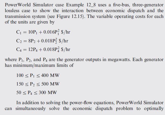
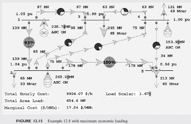
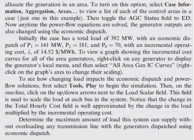
PowerWorld Simulator case Example 12_8 uses a five-bus, three-generator lossless case to show the interaction between economic dispatch and the transmission system (see Figure 12.15). The variable operating costs for each of the units are given by C = 10P] +0.016P $/hr C2=8P2 +0.018P $/hr C4 = 12P4 +0.018P $/hr where P1, P2, and P4 are the generator outputs in megawatts. Each generator has minimum/maximum limits of 100 Pi400 MW 150 P2500 MW 50 P4300 MW In addition to solving the power-flow equations, PowerWorld Simulator can simultaneously solve the economic dispatch problem to optimally