Using LP OPF with PowerWorld Simulator case Example 6_23, plot the variation in the bus 5 marginal price as the Load Scalar is increased from 1.0 in steps of 0.02. What is the maximum possible load scalar without overloading any transmission line? Why is it impossible to operate without violations above this value?

Example 6_23

PowerWorld Simulator case Example 6_23 duplicates the five-bus case from Example 6.20, except that the case is solved using PowerWorld Simulator's LP OPF algorithm (see Figure 6.21). To turn on the OPF option, first select Case Information, Aggregation, Areas..., and toggle the AGC Status field to OPF. Then, rather than solving the case with the "Single Solution" button, select Add-ons, Primal LP to solve using the LP OPF. Initially the OPF solution matches the ED solution from Example 6.20 since there are no overloaded lines. The greencolored fields on the screen immediately to the right of the buses show the marginal cost of supplying electricity to each bus in the system (i.e., the bus LMPs). With the system initially unconstrained, the bus marginal prices are all identical at \(\$ 14.5 / \mathrm{MWh}\), with a Load Scalar of 1.0.
Now increase the Load Scalar field from 1.00 to the maximum economic loading value, determined to be 1.67 in Example 6.20, and again select Add-ons, Primal LP. The bus marginal prices are still all identical, now at a value of \(\$ 17.5 / \mathrm{MWh}\), and with the line from bus 2 to 5 just reaching its maximum value. For load scalar values above 1.67, the line from bus 2 to bus 5 becomes constrained, with a result that the bus marginal prices on the constrained side of the line become higher than those on the unconstrained side.

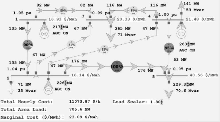
With the load scalar equal to 1.80 , numerically verify that the price of power at bus 5 is approximately \(\$ 40.60 / \mathrm{MWh}\).

1.05 pu 1 135 MW 2 90% 135 MW 1.04 pu 82 MW 67 MW 71 MW 35 Mvar 59% MVA 16.93 $/MWh Total Hourly Cost: Total Area Load: 47 MW 217 MW 67 MW AGC ON 61% MVA 82 MW AGC ON 3 226 MW 176 MW 16.14 $/MWh 0.99 pu 116 MW 11073.87 $/h 705.6 MW Marginal Cost ($/MWh): 23.09 $/MWh 52% 54%- 20.33 $/MWh 265 MW 71 Mvar 100% 116 MW 47 MW 176 MW 5 1.00 pu Load Scalar: 1.80 95% MVA 141 MW 53 Mvar 21.48 $/MWh 263 MW AGC ON 53 MW 0.95 pu 40.56 $/MWh 229.34MW 70.6 Mvar