Resolve Example 6.20, except with the generation at bus 2 set to a fixed value (i.e., modeled as off of Automatic Generation Control). Plot the variation in the total hourly cost as the generation at bus 2 is varied between 1000 and 200 MW in 5 MW steps, resolving the economic dispatch at each step. What is the relationship between bus 2 generation at the minimum point on this plot and the value from economic dispatch in Example 6.20? Assume a Load Scalar of 1.0.

Example 6.20

PowerWorld Simulator case Example 6_20 uses a five-bus, three-generator lossless case to show the interaction between economic dispatch and the transmission system (see Figure 6.19). The variable operating costs for each of the units are given by

\(\mathrm{C}_{1}=10 \mathrm{P}_{1}+0.016 \mathrm{P}_{1}^{2} \$ / \mathrm{hr}\)

\(\mathrm{C}_{2}=8 \mathrm{P}_{2}+0.018 \mathrm{P}_{2}^{2} \$ / \mathrm{hr}\)

\(\mathrm{C}_{4}=12 \mathrm{P}_{4}+0.018 \mathrm{P}_{4}^{2} \$ / \mathrm{hr}\)

where \(\mathrm{P}_{1}, \mathrm{P}_{2}\), and \(\mathrm{P}_{4}\) are the generator outputs in megawatts. Each generator has minimum/maximum limits of

\(100 \leq \mathrm{P}_{1} \leq 400 \mathrm{MW}\)

\(150 \leq \mathrm{P}_{2} \leq 500 \mathrm{MW}\)

\(50 \leq \mathrm{P}_{4} \leq 300 \mathrm{MW}\)

In addition to solving the power flow equations, PowerWorld Simulator can simultaneously solve the economic dispatch problem to optimally allocate the generation in an area. To turn on this option, select Case Information, Aggregation, Areas... to view a list of each of the control areas in a case (just one in this example). Then toggle the AGC Status field to ED. Now anytime the power flow equations are solved, the generator outputs are also changed using the economic dispatch.

Initially, the case has a total load of \(392 \mathrm{MW}\) with an economic dispatch of \(\mathrm{P}_{1}=141 \mathrm{MW}, \mathrm{P}_{2}=181\), and \(\mathrm{P}_{4}=70\), and an incremental operating cost, \(\lambda\), of 14.52 \$/MWh. To view a graph showing the incremental cost curves for all of the area generators, right-click on any generator to display the generator's local menu, and then select All Area Gen IC Curves (right-click on the graph's axes to change their scaling).

To see how changing the load impacts the economic dispatch and power flow solutions, first select Tools, Play to begin the simulation. Then, on the oneline, click on the up/down arrows next to the Load Scalar field. This field is used to scale the load at each bus in the system. Notice that the change in the Total Hourly Cost field is well approximated by the change in the load multiplied by the incremental operating cost.

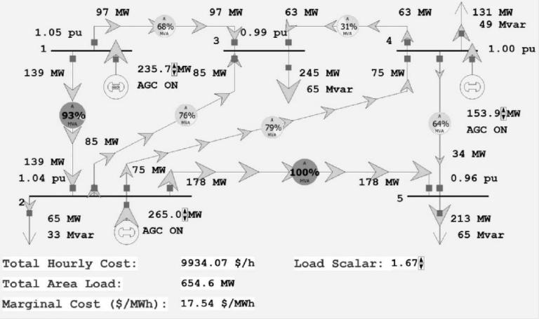
Determine the maximum amount of load this system can supply without overloading any transmission line with the generators dispatched using economic dispatch.

Transcribed Image Text:

1.05 pu 1 139 MW 2 93% HVA 139 MW 1.04 pu 97 MW 85 MW 65 MW 33 Mvar 68% MVA 75 MW 235.7 MW 85 MW AGC ON Total Hourly Cost: Total Area Load: 76% MIA 97 MW 3 265.0 MW AGC ON 178 MW 9934.07 $/h 654.6 MW Marginal Cost ($/MWh): 17.54 $/MWh 0.99 pu 63 MW 79% 245 MW 31% M/K 65 Mvar 100% MVA 63 MW 75 MW 178 MW 5 Load Scalar: 1.67 64% MVA 131 MW 49 Mvar 1.00 pu 153.9 MW AGC ON 34 MW 0.96 pu 213 MW 65 Mvar