New Semester Started
Get
50% OFF
Study Help!
--h --m --s
Claim Now
Question Answers
Textbooks
Find textbooks, questions and answers
Oops, something went wrong!
Change your search query and then try again
S
Books
FREE
Study Help
Expert Questions
Accounting
General Management
Mathematics
Finance
Organizational Behaviour
Law
Physics
Operating System
Management Leadership
Sociology
Programming
Marketing
Database
Computer Network
Economics
Textbooks Solutions
Accounting
Managerial Accounting
Management Leadership
Cost Accounting
Statistics
Business Law
Corporate Finance
Finance
Economics
Auditing
Tutors
Online Tutors
Find a Tutor
Hire a Tutor
Become a Tutor
AI Tutor
AI Study Planner
NEW
Sell Books
Search
Search
Sign In
Register
study help
business
business statistics
The Practice Of Statistics In The Life Sciences 4th Edition Brigitte Baldi, David S. Moore - Solutions
3.20 In Exercise 3.18 you calculated a correlation for knee height (x, in cm) and height (y, in cm). If, instead, you used height (in cm) as the x variable and knee height (in cm) as the y variable, the new correlation woulda. have the inverse value (1 over).b. have the opposite value (a different
3.19 In Exercise 3.18, both heights are measured in centimeters. Just for the fun of it, someone decides to measure knee height in millimeters and height in meters. The data in these units are Knee height x (mm) 577 474 435 448 552 Overall height y (m) 1.921 1.533 1.464 1.627 1.691 The correlation
3.18 Because elderly people may have difficulty standing straight to have their height measured, a study looked at the relationship between overall height and height to the knee. Here are data (in centimeters) for five elderly men:Knee height x (cm) 57.7 47.4 43.5 44.8 55.2 Overall height y (cm)
3.17 If mothers were always 2 years younger than the fathers of their children, the correlation between the ages of mothers and fathers would bea. 1.b. 0.5.c. Can’t tell without seeing the data.
3.16 What are all the values that a correlation r can possibly take?a. r≥0b. 0≤r≤1c. -1≤r≤1
3.15 In Figure 3.6, one child clearly falls outside the overall pattern of the scatterplot and, therefore, might be an outlier. This possible outlier is the child witha. age 42 months and score 57.b. age 26 months and score 71.c. age 17 months and score 121.
3.14 Figure 3.6 is a scatterplot of the age (in months) at which a child begins to talk and the child’s later score on a test of mental ability (Gesell Adaptive Score), for each of 21 children (2 sets of 2 children happen to have the same values).12 To describe the relationship in Figure 3.6, you
3.13 Many species exhibit some degree of sexual dimorphism. Researchers examining the relationship between length and weight in a species of scorpion, Centruroides vittatus, should create a scatterplot of length and weight11a. with different symbols for male and female scorpions.b. for all
3.12 You have data for many individuals on their walking speed and their heart rate after a 10-minute walk. You expect to seea. a positive association.b. very little association.c. a negative association.
3.11 You have data for many individuals on their walking speed and their heart rate after a 10-minute walk. When you make a scatterplot, the explanatory variable on the x axisa. is walking speed.b. is heart rate.c. doesn’t matter.
3.10 Chickadee alarm calls, continued. Exercise 3.5 gives data on the number of D notes per chickadee warning call for predators with various wingspans.a. Use your calculator to find the correlation between the number of D notes per call and wingspan.b. The researchers also recorded chickadee calls
3.9 Enzyme activity and temperature, continued. In Exercise 3.4 you made a scatterplot of acid phosphatase activity rate at different temperatures and described the strength of the relationship. If you calculate the correlation based on the data provided in that exercise, you find r=0.81 (check for
3.8 Breakup distress. College freshmen involved in a dating relationship agreed to participate in a nine-month-long study. Every two weeks, participants answered a detailed questionnaire about their relationship and their emotional well-being. Over the course of the study, 26 of the participants
3.7 Do heavier people burn more energy? Metabolic rate—the rate at which the body consumes energy—is important in studies of weight gain, dieting, and exercise. Here are data on the lean body mass and resting metabolic rate for 12 women and 7 men who are subjects in a study of dieting. Lean
3.6 Night watch. Sleeping in an unfamiliar environment can create a sleep disturbance called the first night effect. A sort of watchful sleep may occur if only one brain hemisphere truly exhibits sleep patterns.Researchers investigated asymmetric brain patterns in 11 healthy right-handed subjects
3.5 Chickadee alarm calls. The black-capped chickadee (Poecile atricapilla) is a small songbird commonly found in the northern United States and Canada. Chickadees often live in cooperative flocks, using a complex language to communicate about food sources and predator threats. In an experiment,
3.4 Enzyme activity and temperature. Enzymatic activity is known to be affected by temperature. A study examined the activity rate (in micromoles per second, μmol/s) of the digestive enzyme acid phosphatase in vitro at varying temperatures (measured in kelvins, K).The findings are displayed in the
3.3 Global climate change. In 2015, the United Nations signed a new global climate change agreement in Paris. Around that time, the Pew Research Center conducted an international survey to explore the relationship between the level of concern over climate change and CO2 emissions per capita in each
3.2 Coral reefs. How sensitive to changes in water temperature are coral reefs? To find out, scientists examined data on summer sea-surface temperatures and coral growth per year at locations in the Red Sea.1 What are the explanatory and response variables? Are they categorical or quantitative?
3.1 Explanatory and response variables? In each of the following situations, is it more reasonable to simply explore the relationship between the two variables or to view one of the variables as an explanatory variable and the other as a response variable? In the latter case, which is the
2.42 Elderly health. A study examined the medical records of elderly patients to determine whether there are differences between men and women in their calcium or inorganic phosphorus blood levels (both in millimoles per liter, mmol/l). The data file Large.Calcium contains the data.21a. Make
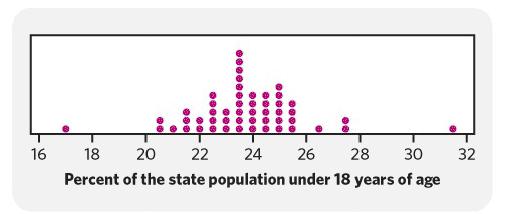
2.41 Young Americans. The dotplot in Figure 1.16 (page 31) displays the distribution of the percents of individuals younger than age 18 in each of the 50 states and the District of Columbia. Note that the values in the dotplot are reported in increments of 0.5 percentage points.a. Give the
2.40 Golden orb weavers. Exercise 2.1 described a study of female golden orb weaver spiders. The study also reported the body mass (in grams) for each of the 21 spiders. Here are the data:0.04 0.11 0.16 0.07 0.13 0.1 0.17 0.25 0.36 0.33 0.29 0.14 0.32 0.57 0.31 0.79 0.49 0.64 0.6 0.99 0.81a. Give
2.39 Aggression and social status in macaque monkeys. The boxplots in Figure 2.9 summarize the number of aggressive behaviors directd at female macaque monkeys of differing social status living in experimentally arranged groups.20 These are modified boxplots that indicate suspected outliers by a
2.38 Mercury levels, continued. In Exercise 2.4 you obtained the fivenumber summary of the distribution of blood mercury levels among 4134 pregnant British women enrolled in a scientific study.a. Use the 1.5×IQR rule to determine whether the smallest and the largest values quoted qualify as
2.37 Logging in the rainforest. “Conservationists have despaired over destruction of tropical rainforest by logging, clearing, and burning.” These words begin a report on a statistical study of the effects of logging in Borneo.19 Researchers compared forest plots that had never been logged
2.36 Daily activity and obesity. People gain weight when they take in more energy from food than they expend. Table 2.1 compares volunteer subjects who were lean with others who were mildly obese. None of the subjects followed an exercise program. The subjects wore sensors that recorded every move
2.35 Cicadas as fertilizer? Every 17 years, swarms of cicadas emerge from the ground in the eastern United States, live for about six weeks, then die. (There are several “broods,” so we see cicada eruptions more often than every 17 years.) So many cicadas die that their bodies may serve as
2.34 Does breastfeeding weaken bones? Breastfeeding mothers secrete calcium into their milk. Some of the calcium may come from their bones, so mothers may lose bone mineral content. Researchers compared 47 breastfeeding women with 22 women of similar age who were neither pregnant nor lactating.
2.33 A standard deviation contest. This is a standard deviation contest.You must choose four numbers from the whole numbers 0 to 10, with repeats allowed.a. Choose four numbers that have the smallest possible standard deviation.b. Choose four numbers that have the largest possible standard
2.32 Guinea pig survival times. Here are the survival times (in days) of 72 guinea pigs after they were injected with infectious bacteria in a medical experiment:15 43 45 53 56 56 57 58 66 67 73 74 79 80 80 81 81 81 82 83 83 84 88 89 91 91 92 92 97 99 99 100 100 101 102 102 102 103 104 107 108 109
2.31 Nanomedicine. In Exercise 1.41 (page 36) you graphed the distribution of ovarian tumor increases under two experimental conditions:a new nanoparticle-based delivery system for a suicide gene therapy or an inactive buffer solution.a. Make a boxplot comparing tumor increase under the two
2.30 Behavior of the median. Place five observations on the line in the Mean and Median applet by clicking below it.a. Add one additional observation without changing the median. Where is your new point?b. Use the applet to convince yourself that when you add yet another observation (there are now
2.29 Metabolic rate. In Example 2.7 you examined the metabolic rates of 7 men. Here are the metabolic rates for 12 women from the same study:995 1425 1396 1418 1502 1256 1189 913 1124 1052 1347 1204a. The most common methods for formal comparison of two groups use x̄and s to summarize the data.
2.28 Laughing behavior. A study of freely forming groups in bars throughout Europe examined the number of individuals found in groups whose members were laughing together. The study reported on a total of 501 laughing groups, distributed as follows:14 Number of individuals in group 2 3 4 5 6 Number
2.27 Anorexia nervosa. Figure 1.9 (page 20) is a histogram of the distribution of age at onset of anorexia for 691 Canadian girls diagnosed with the disorder. If you round the age to whole numbers of years, the first bar of the histogram (the first class) would include all girls diagnosed during
2.26 Making resistance visible. In the Mean and Median applet, place three observations on the line by clicking below it: two close together near the center of the line, and one somewhat to the right of these two.a. Pull the single rightmost observation out to the right. (Place the cursor on the
2.25 Lyme disease. Figure 1.8 (page 19) shows the age in years of 241,931 patients diagnosed with Lyme disease in the United States between 1992 and 2006. Give a brief description of the important features of the distribution. Explain why no numerical summary would appropriately describe this
2.24 Food oils and health. Table 1.2 (page 34) gives the ratio of omega-3 to omega-6 fatty acids in common food oils. Exercise 1.36 asked you to plot the data. The distribution is strongly right-skewed with a high outlier.Do you expect the mean to be greater than the median, about equal to the
2.23 Which of the following is least affected if an extreme high outlier is added to your data?a. the medianb. the meanc. the standard deviation
2.22 What are the correct units for the standard deviation of the 15 cesium-137 values in Exercise 2.14?a. no units—it’s just a numberb. becquerels per kilogram of dry tissuec. becquerels squared per square kilogram of dry tissue
2.21 What is the approximate value of the standard deviation of the 15 cesium-137 values in Exercise 2.14? (Use your calculator.)a. 1.47b. 1.52c. 2.32
2.20 What are all the values that a standard deviation s can possibly take?a. 0≤sb. 0≤s≤1c. -1≤s≤1
2.19 To make a boxplot of a distribution, you must knowa. all the individual observations.b. the mean and the standard deviation.c. the five-number summary.
2.18 What percent of the observations in a distribution lie between the first quartile and the third quartile?a. 25%b. 50%c. 75%
2.17 Ifa distribution is clearly skewed to the right,a. the mean is less than the median.b. the mean and the median are equal.c. the mean is greater than the median.
2.16 (Optional) What is the interquartile range, IQR, of the data in Exercise 2.14?a. 1.3b. 2.0c. 2.3
2.15 What is the median of the data in Exercise 2.14?a. 5.70b. 6.00c. 6.28
2.14 Cesium-137 is a waste product of nuclear reactors. A study examined the cesium-137 tissue concentration of a random sample of 15 Pacific bluefin tuna, Thunnus orientalis, captured off the coast of California four months after the Fukushima (Japan) nuclear reactor meltdown of 2011.Here are the
2.13 Highly Superior Autobiographical Memory, continued.The study in Example 2.11 assessed common obsessional symptoms in the HSAM and the control individuals, as previous findings had suggested a possible obsessional component to HSAM.The study participants completed the Leyton Obsessional
2.12 Temperatures records. In Exercise 1.14 (page 28) you downloaded historical temperature records for Los Angeles from NASA’s website, and examined the distribution of meteorological annual mean temperatures (“metANN” column, in degrees Celsius, °C).a. Obtain the mean and the median for
2.11 Blood pressure readings. A manufacturer of blood pressure monitoring devices lists 10 factors that can affect blood pressure readings:11 1. Blood pressure cuff too small 2. Blood pressure cuff used over clothing 3. Not resting for a few minutes 4. Arms, back, or feet unsupported 5. Emotional
2.10 Glucose levels, continued. In Exercise 2.6 you made side-by-side boxplots comparing the group and individual training methods for diabetes control. Use the 1.5×IQR rule to identify any suspected outliers. Then look at the raw data to determine if unusually high or low values in either data
2.9 Spider silk, continued. In Exercise 2.1 you plotted the silk yield stress for 21 female golden orb weaver spiders. Use the 1.5×IQR rule to identify suspected outliers.
2.8 x̄ and s are not enough. The mean x¯ and standard deviation s measure center and spread but are not a complete description of a 151 distribution. Data sets with different shapes can have the same mean and standard deviation. To demonstrate this fact, use your calculator to find x¯ and s for
2.7 The cost of common blood tests. A 2014 study examined the prices(in dollars) billed by hospitals all over California for common blood tests such as a blood lipid panel (to check cholesterol level, first row)and a blood metabolic panel (including fasting plasma glucose level, second row). Here
2.5 Spider silk, continued. In Exercise 2.1 you plotted the silk yield stress for 21 female golden orb weaver spiders.a. Obtain the five-number summary of the distribution of yield stresses.b. Obtain the mean and the standard deviation of the sample of yield stresses.c. Which summary gives more
2.4 Mercury levels in pregnant women. A study recorded the blood mercury levels (in micrograms per liter, μg/l) of 4134 pregnant British women enrolled in the Avon Longitudinal Study of Parents and Children.8 The published findings include the following statement:“Blood mercury levels ranged
2.3 Age of participants, summarized. A study of a new type of vision screening test recruited a sample of 175 children age 3 to 7 years. The publication provides the following summary of the children’s ages:“Twelve patients (7%) were 3 years old; 33 (19%), 4 years old; 29(17%), 5 years old; 69
2.2 Deep-sea sediments. Phytopigments are markers of the amount of organic matter that settles in sediments on the ocean floor.Phytopigment concentrations in deep-sea sediments collected worldwide showed a very strong right-skew.5 Of two summary statistics, 0.015 and 0.009 gram per square meter of
2.1 Spider silk. Spider silk is the strongest known material, natural or man-made, on a weight basis. A study examined the mechanical properties of spider silk using 21 female golden orb weavers, Nephila clavipes. Here are data on silk yield stress, which represents the amount of force per unit
1.45 Everglades. Everglades National Park is the largest subtropical wilderness in the United States and has been designated a Wetland of International Importance. This important ecosystem is closely monitored by the U.S. Geological Survey. The Large.Everglades data file contains data on five
1.44 Exercising. The Gallup polling organization interviews samples of individuals to learn about public opinions and habits. One question Gallup asks regularly of randomly picked Americans is whether they exercised for at least 30 minutes on three or more of the past seven days. Figure 1.19 is a
1.43 Herbicide resistance in weeds. Farmers use herbicides to limit the growth of weeds among their crops. Eventually, this technique places evolutionary pressure on weed species, resulting in herbicide resistance.The International Survey of Herbicide Resistant Weeds keeps track of documented cases
1.42 Fur seals on Saint George Island, continued. Make a time plot of the number of fur seals born per year from Exercise 1.40. What does the time plot show that your plot in Exercise 1.40 does not show? When you have data collected over time, a time plot is often needed to understand what is
1.41 Nanomedicine. Researchers examined a new treatment for advanced ovarian cancer in a mouse model. They created a nanoparticle-based delivery system for a suicide gene therapy to be delivered directly to the tumor cells. The grafted tumors were injected either with the new treatment or with only
1.40 Fur seals on Saint George Island. Every year hundreds of thousands of northern fur seals return to their haul-out territory in the Pribilof Islands in Alaska to breed, give birth, and teach their pups to swim, hunt, and survive in the Bering Sea. U.S. commercial fur sealing operations ended in
1.39 Stemplots: Flower length. Here are the flower lengths (in millimeters) of 16 specimens of the tropical plant Heliconia bihai.31 46.3 46.4 46.6 46.7 46.8 46.8 46.9 47.1 47.1 47.4 48.1 48.2 48.3 48.4 50.1 50.3a. Follow the model in Exercise 1.37 to create a stemplot of these flower lengths.b.
1.38 Data maps: Obesity. The CDC studies the obesity crisis in the United States by obtaining the body mass index (BMI, from self-reported weight and height) of representative sets of individuals. A person is considered obese if his or her BMI exceeds 30. Table 1.3 reports the percent of adults in
1.37 Stemplots: Healing time. Biologists studying the healing of skin wounds measured the rate at which new cells closed a razor cut made to the skin of an anesthetized newt. Here are the sorted data from 18 newts, measured in micrometers per hour:29 11 12 14 18 22 22 23 23 26 27 28 29 30 33 34 35
1.36 Food oils and health. Fatty acids, despite their unpleasant name, are necessary for human health. Two types of essential fatty acids, called omega-3 and omega-6, are not produced by our bodies and so must be obtained from our food. Food oils, which are widely used in food processing and
1.35 Acid rain. Changing the choice of classes can change the appearance of a histogram. Here is an example in which a small shift in the classes, with no change in the number of classes, has an important effect on the histogram. The data are the acidity levels (measured by pH) in 105 samples of
1.34 Highly Superior Autobiographical Memory, continued. The researchers in Exercise 1.32 also administered the quiz of past public events to 30 individuals who did not claim to have any unusual memory abilities (controls). Their scores are displayed in Figure 1.17(b), using the same horizontal
1.33 Which graph? Of the following data sets, which would you display with a bar graph and which would you display with a histogram? Explain why.a. A record of the gender of selected individuals (labeled as male = 0, female = 1)b. A record of the age of selected parents (in years) at birth of first
1.32 Do you have Highly Superior Autobiographical Memory? Some individuals have the ability to recall accurately vast amounts of autobiographical information without mnemonic tricks or extra practice.This ability is called HSAM, for Highly Superior Autobiographical Memory. A research team
1.31 More on the overweight problem. The same NCHS report (see Exercise 1.30) breaks down the sampled individuals by age group. Here are the percents of obese individuals in the 2011 survey for each age group:Age group Percent who are obese 18 to 44 26.2 45 to 64 32.2 65 to 74 31.6 75 and over
1.30 The overweight problem. The 2011 National Health Interview Survey by the National Center for Health Statistics (NCHS) provides weight categorizations for adults 18 years and older based on their body mass index:Weight category Percent of adults Underweight 1.6 Healthy weight 36.3 Overweight
1.29 Manatee deaths. Manatees are an endangered species of herbivorous, aquatic mammals found primarily in the rivers and estuaries of Florida. As part of its conservation efforts, the Florida Fish and Wildlife Commission records the cause of death for every recovered manatee carcass. Here is a
1.28 Deaths among young people. Here are the number of deaths among persons aged 15 to 24 years in the United States in 2010 due to the leading causes of death for this age group: accidents, 12,015; homicide, 4651;suicide, 4559; cancer, 1594; heart disease, 984; congenital defects, 401.24a. Make
1.27 Mercury in lakes. Mercury is a metal that is highly toxic to the nervous system. Following is a small part of an EESEE data set (“Mercury in Bass”) from a study that assessed the water quality of 53 representative lakes in Florida:23 Lake name PH Chlorophyll (mg/l) Avg. mercury in fish
1.26 Eating habits. You are preparing to study the eating habits of elementary schoolchildren. Describe two categorical variables and two quantitative variables that you might record for each child. Give the units of measurement for the quantitative variables.
1.25 Endangered species. Bald eagles are an endangered bird species suffering from loss of habitat and pesticide contamination of rivers. A field biologist studying the reproduction of bald eagles records data for the following variables. Which of these variables are categorical, and which are
1.24 The shape of the distribution in the previous exercise isa. strongly skewed to the right.b. roughly symmetric.c. strongly skewed to the left.
1.23 The 2010 U.S. census reported the percent of individuals younger than age 18 in each of the 50 states and the District of Columbia. The data are shown in a doplot in Figure 1.16. This distribution isa. single-peaked without outliers.b. single-peaked with two outliers.c. multiple-peaked with
1.22 The shape of the distribution of takeoff angles in Figure 1.15 isa. skewed to the right.b. roughly symmetric.c. skewed to the left.
1.21 What percent of jumps have a takeoff angle of 35 degrees or less?a. 8%b. 16%c. 31%
1.20 Which of the following conclusions can be reached from Figure 1.14?a. The majority of adults who are overweight and obese live in highincome countries.b. The majority of adults who live in high-income countries are overweight and obese.c. Both conclusions are correct.Figure 1.15 is a histogram
1.19 The graph in Figure 1.14 isa. a bar graph that can be made into one pie chart.b. a bar graph that cannot be made into one pie chart.c. a histogram with a clear right skew.
1.18 Kidney transplants represented what percent of single-organ transplants in 2010?a. Nearly 61%b. One-sixth (nearly 17%)c. This percent cannot be calculated from the information provided in the table.
1.17 The data on single-organ transplants can be displayed ina. a pie chart but not a bar graph.b. a bar graph but not a pie chart.c. either a pie chart or a bar graph.
1.16 The two variables in the Arkansas study area. both categorical variables.b. both quantitative variables.c. one categorical variable and one quantitative variable.The Statistical Abstract of the United States, prepared by the Census Bureau, provides the number of single-organ transplants for
1.15 A study of a very large number of pregnant women in Arkansas reports that the women gained, on average, 14 pounds during their pregnancy and that 18% of the women smoked.20 Which of the following is not a variable in this study?a. Pregnancy statusb. Smoking statusc. Weight gain
1.14 Temperatures records. NASA’s Goddard Institute for Space Studies (GISS) allows you to download historical temperature records for locations worldwide. Go to http://data.giss.nasa.gov/gistemp/station_data, scroll down to“Download Station Data,” and type “Los Angeles.” (You may be
1.13 Student data. Consider gathering some basic information about your classmates, perhaps during lecture or discussion.a. You may be interested in the distribution of student heights.Which type of variable is student height? Explain how you would collect the data if the class had 30 or 40
1.12 Atmospheric CO2 levels. Elevated atmospheric CO2 levels have been linked to global warming. The Mauna Loa Observatory in Hawaii has the longest record of direct measurements of CO2 in the atmosphere, going back to 1958. Figure 1.13 shows the trends in monthly atmospheric CO2 levels over Hawaii
1.11 Opioid pain relievers. In Exercise 1.5, we looked at state prescription rates for opioid pain relievers. Here are the number of deaths from prescription opioid pain relievers in the United States in the years 2000 to 2014:17Make a time plot of these data and describe the trend that your plot
1.10 Glucose levels. People with diabetes must monitor and control their blood glucose level. The goal is to maintain “fasting plasma glucose” between about 90 and 130 milligrams per deciliter (mg/dl).A study planned to compare the effectiveness of group instruction versus individual
1.9 California pertussis epidemic. In Example 1.7 we used a histogram to display the rates of pertussis cases per 100,000 persons in each of the 59 California counties for all of 2014. Create a dotplot of the data, by hand or using software. Compare your dotplot to the histogram in Figure 1.7 and
1.8 Age of onset for anorexia nervosa. Anorexia nervosa is an eating disorder characterized, in part, by the fear of becoming fat and by voluntary starvation; it often leads to death from suicide or organ failure. A Canadian study surveyed 691 adolescent girls diagnosed with anorexia nervosa and
1.7 Prescriptions of opioid pain relievers. In Exercise 1.5, you made a histogram of the state prescription rates for opioid pain relievers.Would you say that the distribution is single-peaked or multiplepeaked?Is it roughly symmetric or skewed?
Showing 100 - 200
of 6970
1
2
3
4
5
6
7
8
9
10
11
12
13
14
15
Last
Step by Step Answers