New Semester
Started
Get
50% OFF
Study Help!
--h --m --s
Claim Now
Question Answers
Textbooks
Find textbooks, questions and answers
Oops, something went wrong!
Change your search query and then try again
S
Books
FREE
Study Help
Expert Questions
Accounting
General Management
Mathematics
Finance
Organizational Behaviour
Law
Physics
Operating System
Management Leadership
Sociology
Programming
Marketing
Database
Computer Network
Economics
Textbooks Solutions
Accounting
Managerial Accounting
Management Leadership
Cost Accounting
Statistics
Business Law
Corporate Finance
Finance
Economics
Auditing
Tutors
Online Tutors
Find a Tutor
Hire a Tutor
Become a Tutor
AI Tutor
AI Study Planner
NEW
Sell Books
Search
Search
Sign In
Register
study help
business
statistical techniques in business
Data Science And Machine Learning Mathematical And Statistical Methods 1st Edition Dirk P. Kroese, Thomas Taimre, Radislav Vaisman, Zdravko Botev - Solutions
Let \(\mathscr{G}\) be an RKHS with reproducing kernel \(\kappa\). Show that \(\kappa\) is a positive semidefinite function.
Show that a reproducing kernel, if it exists, is unique.
Let \(\mathscr{G}\) be a Hilbert space of functions \(g: \mathscr{X} \rightarrow \mathbb{R}\). Recall that the evaluation functional is the map \(\delta_{x}: g \mapsto g(\boldsymbol{x})\) for a given \(\boldsymbol{x} \in \mathscr{X}\). Show that evaluation functionals are linear operators.
Let \(\mathscr{G}_{0}\) be the pre-RKHS \(\mathscr{G}_{0}\) constructed in the proof of Theorem 6.2. Thus, \(g \in \mathscr{G}_{0}\) is of the form \(g=\sum_{i=1}^{n} \alpha_{i} \kappa_{x_{i}}\) and\[ \left\langle g, \kappa_{\boldsymbol{x}}\rightangle_{\mathscr{G}_{0}}=\sum_{i=1}^{n}
Continuing Exercise 4 , let \(\left(f_{n}\right)\) be a Cauchy sequence in \(\mathscr{G}_{0}\) such that \(\left|f_{n}(\boldsymbol{x})\right| \rightarrow 0\) for all \(\boldsymbol{x}\). Show that \(\left\|f_{n}\right\|_{\mathscr{G}_{0}} \rightarrow 0\).
Continuing Exercises 5 and 4, to show that the inner product (6.14) is well defined, a number of facts have to be checked.(a) Verify that the limit converges.(b) Verify that the limit is independent of the Cauchy sequences used.(c) Verify that the properties of an inner product are satisfied. The
Exercises 4-6 show that \(\mathscr{G}\) defined in the proof of Theorem 6.2 is an inner product space. It remains to prove that \(\mathscr{G}\) is an RKHS. This requires us to prove that the inner product space \(\mathscr{G}\) is complete (and thus Hilbert), and that its evaluation functionals are
If \(\kappa_{1}\) and \(\kappa_{2}\) are kernels on \(\mathscr{X}\) and \(\mathscr{Y}\), then \(\kappa_{+},\left((\boldsymbol{x}, \boldsymbol{y}),\left(\boldsymbol{x}^{\prime}, \boldsymbol{y}^{\prime}\right)\right):=\kappa_{1}\left(\boldsymbol{x},
An RKHS enjoys the following desirable smoothness property: if \(\left(g_{n}\right)\) is a sequence belonging to RKHS \(\mathscr{G}\) on \(\mathscr{X}\), and \(\left\|g_{n}-g\right\|_{\mathscr{G}} \rightarrow 0\), then \(g(\boldsymbol{x})=\lim _{n} g_{n}(\boldsymbol{x})\) for all \(\boldsymbol{x}
Let \(\mathbf{X}\) be an \(\mathbb{R}^{d}\)-valued random variable that is symmetric about the origin (that is, \(\boldsymbol{X}\) and \((-\boldsymbol{X})\) are identically distributed). Denote by \(\mu\) is its distribution and \(\psi(\boldsymbol{t})=\) \(\mathbb{E} \mathrm{e}^{i
Suppose an \(\mathrm{RKHS} \mathscr{G}\) of functions from \(\mathscr{X} \rightarrow \mathbb{R}\) (with kernel \(\kappa\) ) is invariant under a group \(\mathscr{T}\) of transformations \(T: \mathscr{X} \rightarrow \mathscr{X}\); that is, for all \(f, g \in \mathscr{G}\) and \(T \in \mathscr{T}\),
Given two Hilbert spaces \(\mathscr{H}\) and \(\mathscr{G}\), we call a mapping \(A: \mathscr{H} \rightarrow \mathscr{G}\) a Hilbert space isomorphism if it is (i) a linear map; that is, \(A(a f+b g)=a A(f)+b A(g)\) for any \(f, g \in \mathscr{H}\) and a, \(b \in \mathbb{R}\).(ii) a surjective
Let \(\mathbf{X}\) be an \(n \times p\) model matrix. Show that \(\mathbf{X}^{\top} \mathbf{X}+n \gamma \mathbf{I} \mathbf{I}_{p}\) for \(\gamma>0\) is invertible.
As Example 6.8 clearly illustrates, the pdf of a random variable that is symmetric about the origin is not in general a valid reproducing kernel. Take two such iid random variables \(X\) and \(X^{\prime}\) with common pdf \(f\), and define \(Z=X+X^{\prime}\). Denote by \(\psi_{z}\) and \(f_{Z}\)
For the smoothing cubic spline of Section 6.6, show that \(\kappa(x, u)=\frac{\max \{x, u\} \min \{x, u\}^{2}}{2}-\frac{\min \{x, u\}^{3}}{6} .\).
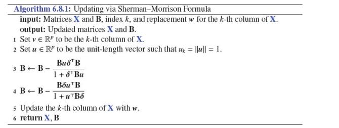
Let \(\mathbf{X}\) be an \(n \times p\) model matrix and let \(\boldsymbol{u} \in \mathbb{R}^{p}\) be the unit-length vector with \(k\)-th entry equal to one \(\left(u_{k}=\|\boldsymbol{u}\|=1\right)\). Suppose that the \(k\)-th column of \(\mathbf{X}\) is \(\boldsymbol{v}\) and that it is replaced
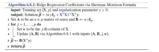
Use Algorithm 6. 8.1 from Exercise 16 to write Python code that computes the ridge regression coefficient \(\boldsymbol{\beta}\) in (6.5) and use it to replicate the results on Figure 6.1. The following pseudo-code (with running cost of \(O\left((n+p) p^{2}\right)\) ) may help with the writing of
Consider Example 2.10 with \(\mathbf{D}=\operatorname{diag}\left(\lambda_{1}, \ldots, \lambda_{p}\right)\) for some nonnegative vector \(\lambda \in \mathbb{R}^{p}\), so that twice the negative logarithm of the model evidence can be written as\[ -2 \ln g(\boldsymbol{y})=l(\boldsymbol{\lambda}):=n
(Exercise 18 continued.) Consider again Example 2.10 with \(\mathbf{D}=\operatorname{diag}\left(\lambda_{1}, \ldots, \lambda_{p}\right)\) for some nonnegative model-selection parameter \(\lambda \in \mathbb{R}^{p}\). A Bayesian choice for \(\lambda\) is the maximizer of the marginal likelihood
In this exercise we explore how the early stopping of the gradient descent iterations (see Example B.10),\[ \boldsymbol{x}_{t+1}=\boldsymbol{x}_{t}-\alpha abla f\left(\boldsymbol{x}_{t}\right), \quad t=0,1, \ldots \]is (approximately) equivalent to the global minimization of
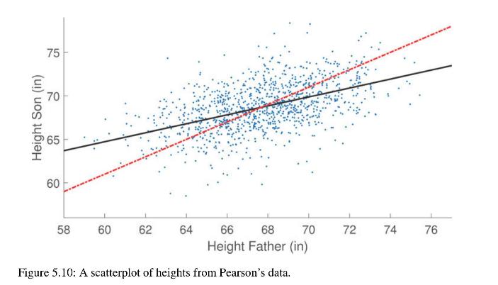
Following his mentor Francis Galton, the mathematician/statistician Karl Pearson conducted comprehensive studies comparing hereditary traits between members of the same family. Figure 5.10 depicts the measurements of the heights of 1078 fathers and their adult sons (one son per father). The data is
For the simple linear regression model, show that the values for \(\widehat{\beta_{1}}\) and \(\widehat{\beta_{0}}\) that solve the equations (5.9) are:\[ \begin{gather*} \widehat{\beta_{1}}=\frac{\sum_{i=1}^{n}\left(x_{i}-x\right)\left(y_{i}-y\right)}{\sum_{i=1}^{n}\left(x_{i}-x\right)^{2}}
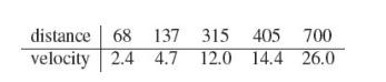
Edwin Hubble discovered that the universe is expanding. If \(v\) is a galaxy's recession velocity (relative to any other galaxy) and \(d\) is its distance (from that same galaxy), Hubble's law states that\[ v=H d \]where \(H\) is known as Hubble's constant. The following are distance (in millions
The multiple linear regression model (5.6) can be viewed as a first-order approximation of the general model\[ \begin{equation*} Y=g(\boldsymbol{x})+\varepsilon \tag{5.42} \end{equation*} \]where \(\mathbb{E} \varepsilon=0, \operatorname{Var} \varepsilon=\sigma^{2}\), and \(g(\boldsymbol{x})\)
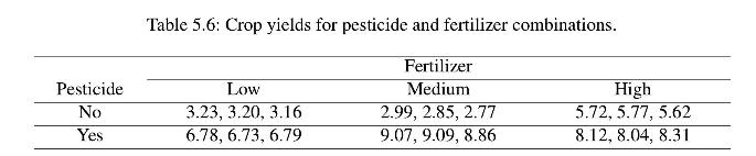
Table 5.6 shows data from an agricultural experiment where crop yield was measured for two levels of pesticide and three levels of fertilizer. There are three responses for each combination.(a) Organize the data in standard form, where each row corresponds to a single measurement and the columns
Show that for the birthweight data in Section 5.6.6.2 there is no significant decrease in birthweight for smoking mothers. [Hint: create a new variable nonsmoke \(=1\)-smoke, which reverses the encoding for the smoking and non-smoking mothers. Then, the parameter \(\beta_{1}+\) \(\beta_{3}\) in the
Prove (5.37) and (5.38).
In the Tobit regression model with normally distributed errors, the response is modeled as:\[ Y_{i}=\left\{\begin{array}{ll} Z_{i}, & \text { if } u_{i}u_{i}} \varphi_{\sigma^{2}}\left(y_{i}-\boldsymbol{x}_{i}^{\top} \boldsymbol{\beta}\right) \times \prod_{i: y_{i}=u_{i}}
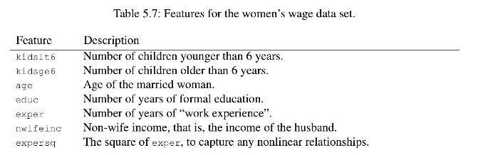
Dowload data set WomenWage.csv from the book's website. This data set is a tidied-up version of the women's wages data set from [91]. The first column of the data (hours) is the response variable \(Y\). It shows the hours spent in the labor force by married women in the 1970s. We want to understand
Let \(\mathbf{P}\) be a projection matrix. Show that the diagonal elements of \(\mathbf{P}\) all lie in the interval \([0,1]\). In particular, for \(\mathbf{P}=\mathbf{X X}^{+}\)in Theorem 5.1, the leverage value \(p_{i}:=\mathbf{P}_{i i}\) satisfies \(0 \leqslant p_{i}\) \(\leqslant 1\) for all
Consider the linear model \(\boldsymbol{Y}=\mathbf{X} \boldsymbol{\beta}+\varepsilon\) in (5.8), with \(\mathbf{X}\) being the \(n \times p\) model matrix and \(\boldsymbol{\varepsilon}\) having expectation vector \(\mathbf{0}\) and covariance matrix \(\sigma^{2} \mathbf{I}_{n}\). Suppose that
Take the linear model \(\boldsymbol{Y}=\mathbf{X} \boldsymbol{\beta}+\varepsilon\), where \(\mathbf{X}\) is an \(n \times p\) model matrix, \(\varepsilon=\mathbf{0}\), and \(\mathbb{C o v}(\boldsymbol{\varepsilon})=\) \(\sigma^{2} \mathbf{I}_{n}\). Let \(\mathbf{P}=\mathbf{X X} \mathbf{X}^{+}\)be
Consider a normal linear model \(\boldsymbol{Y}=\mathbf{X} \boldsymbol{\beta}+\varepsilon\), where \(\mathbf{X}\) is an \(n \times p\) model matrix and \(\varepsilon \sim \mathscr{N}\left(\mathbf{0}, \sigma^{2} \mathbf{I}_{n}\right)\). Exercise 12 shows that for any such model the \(i\)-th
Using the notation from Exercises 11-13, Cook's distance for observation \(i\) is defined as\[ D_{i}:=\frac{\widehat{\boldsymbol{Y}}-\widehat{\boldsymbol{Y}}^{(i)^{2}}}{p S^{2}} \]It measures the change in the fitted values when the \(i\)-th observation is removed, relative to the residual
Prove that if we add an additional feature to the general linear model, then \(R^{2}\), the coefficient of determination, is necessarily non-decreasing in value and hence cannot be used to compare models with different numbers of predictors.
Let \(\boldsymbol{X}:=\left[X_{1} \ldots, X_{n}\right]^{\top}\) and \(\boldsymbol{\mu}:=\left[\mu_{1}, \ldots \mu_{n}\right]^{\top}\). In the fundamental Theorem C.9, we use the fact that if \(X_{i} \sim \mathscr{N}\left(\mu_{i}, 1\right), i=1, \ldots, n\) are independent, then \(\|X\|^{2}\) has
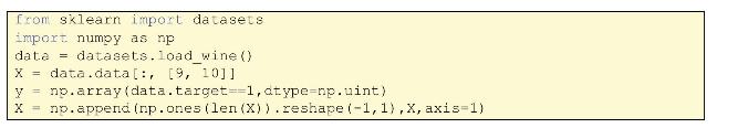
Carry out a logistic regression analysis on a (partial) wine data set classification problem. The data can be loaded using the following code.The model matrix has three features, including the constant feature. Instead of using Newton's method (5.39) to estimate \(\boldsymbol{\beta}\), implement a
Consider again Example5.10, where we train the learner via the Newton iteration (5.39). If \(\mathbf{X}^{\top}:=\left[x_{1}, \ldots, \boldsymbol{x}_{n}\right]\) defines the matrix of predictors and \(\boldsymbol{\mu}_{t}:=\boldsymbol{h}\left(\boldsymbol{X} \boldsymbol{\beta}_{t}\right)\), then the
In multi-output linear regression, the response variable is a real-valued vector of dimension, say, \(m\). Similar to (5.8), the model can be written in matrix notation:\[ \mathbf{Y}=\mathbf{X B}+\begin{gathered} \boldsymbol{\varepsilon}_{1}^{\top} \\ \vdots \\
This exercise is to show that the Fisher information matrix \(\mathbf{F}(\boldsymbol{\theta})\) in (4.8) is equal to the matrix \(\mathbf{H}(\boldsymbol{\theta})\) in (4.9), in the special case where \(f=\mathrm{g}(\cdot \mid \boldsymbol{\theta})\), and under the assumption that integration and
Plot the mixture of \(\mathscr{N}(0,1), \mathscr{U}(0,1)\), and \(\operatorname{Exp}(1)\) distributions, with weights \(w_{1}=w_{2}=w_{3}\) \(=1 / 3\).
Denote the pdfs in Exercise 2 by \(f_{1}, f_{2}, f_{3}\), respectively. Suppose that \(X\) is simulated via the two-step procedure: First, draw \(Z\) from \(\{1,2,3\}\), then \(\operatorname{draw} X\) from \(f_{Z}\). How likely is it that the outcome \(x=0.5\) of \(X\) has come from the uniform
Simulate an iid training set of size 100 from the Gamma \((2.3,0.5)\) distribution, and implement the Fisher scoring method in Example 4.1 to find the maximum likelihood estimate. Plot the true and approximate pdfs.
Let \(\mathscr{T}=\left\{\boldsymbol{X}_{1}, \ldots, \boldsymbol{X}_{n}\right\}\) be iid data from a pdf \(g(\boldsymbol{x} \mid \boldsymbol{\theta})\) with Fisher matrix \(\mathbf{F}(\boldsymbol{\theta})\). Explain why, under the conditions where (4.7) holds,\[
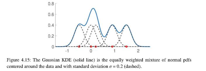
Figure 4.15 shows a Gaussian KDE with bandwidth \(\sigma=0.2\) on the points \(-0.5,0,0.2,0.9\), and 1.5. Reproduce the plot in Python. Using the same bandwidth, plot also the KDE for the same data, but now with \(\phi(z)=1 / 2, z \in[-1,1]\). 0.8 An 0.6 0.4 0.2 0 -1 0 2 Figure 4.15: The Gaussian
For fixed \(x^{\prime}\), the Gaussian kernel function is the solution to Fourier's heat equation \[ \frac{\partial}{\partial t} f(x \mid t)=\frac{1}{2} \frac{\partial^{2}}{\partial x^{2}} f(x \mid t), \quad x \in \mathbb{R}, t>0 \]with initial condition \(f(x \mid
Show that the Ward linkage given in (4.41) is equal to dward (I, J)= == I+I || x-x || 2
Carry out the agglomerative hierarchical clustering of Example 4.8 via the linkage method from scipy.cluster.hierarchy. Show that the linkage matrices are the same. Give a scatterplot of the data, color coded into \(K=3\) clusters.
Suppose that we have the data \(\tau_{\mathrm{n}}=\left\{x_{1}, \ldots, x_{n}\right\}\) in \(\mathbb{R}\) and decide to train the two-component Gaussian mixture model\[ g(x \mid \boldsymbol{\theta})=w_{1} \frac{1}{\sqrt{2 \pi \sigma_{1}^{2}}} \exp \left(-\frac{\left(x-\mu_{1}\right)^{2}}{2
A \(d\)-dimensional normal random vector \(X \sim \mathscr{N}\left(\boldsymbol{\mu}, \sum\right)\) can be defined via an affine transformation, \(\boldsymbol{X}=\boldsymbol{\mu}+\boldsymbol{\Sigma}^{1 / 2} \mathbf{Z}\), of a standard normal random vector \(\boldsymbol{Z} \sim
A generalization of both the gamma and inverse-gamma distribution is the generalized inverse-gamma distribution, which has density\[\begin{equation*}f(s)=\frac{(a / b)^{p / 2}}{2 K_{p}(\sqrt{a b})} s^{p-1} \mathrm{e}^{-\frac{1}{2}(a s+b / s)}, \quad a, b, s>0, \quad p \in \mathbb{R}
In Exercise 11 we viewed the multivariate Student \(\mathbf{t}_{\alpha}\) distribution as a scale-mixture of the \(\mathscr{N}\left(\mathbf{0}, \mathbf{I}_{d}\right)\) distribution. In this exercise, we consider a similar transformation, but now \(\sum^{1 / 2} Z \sim \mathscr{N}\left(0,
Consider the ellipsoid \(E=\left\{\boldsymbol{x} \in \mathbb{R}^{d}: x \boldsymbol{\Sigma}^{-1} \boldsymbol{x}=1\right\}\) in (4.42). Let \(\mathbf{U D}^{2} \mathbf{U}^{\top}\) be an SVD of \(\boldsymbol{\Sigma}\). Show that the linear transformation \(\boldsymbol{x} \mapsto \mathbf{U}^{\top}
Figure 4.13 shows how the centered "surfboard" data are projected onto the first column of the principal component matrix \(\mathbf{U}\). Suppose we project the data instead onto the plane spanned by the first two columns of \(\mathbf{U}\). What are \(a\) and \(b\) in the representation \(a x_{1}+b
Figure 4.14 suggests that we can assign each feature vector \(\boldsymbol{x}\) in the iris data set to one of two clusters, based on the value of \(\boldsymbol{u}_{1}^{\top} \boldsymbol{x}\), where \(\boldsymbol{u}_{1}\) is the first principal component. Plot the sepal lengths against petal lengths
We can modify the Box-Muller method in Example 3.1 to draw \(X\) and \(Y\) uniformly on the unit disc, \(\left\{(x, y) \in \mathbb{R}^{2}: x^{2}+y^{2} \leqslant 1\right\}\), in the following way: Independently draw a radius \(R\) and an angle \(\Theta \sim \mathscr{U}(0,2 \pi)\), and return \(X=R
A simple acceptance-rejection method to simulate a vector \(\boldsymbol{X}\) in the unit \(d\)-ball \(\left\{\boldsymbol{x} \in \mathbb{R}^{d}\right.\) : \(\|x\| \leqslant 1\}\) is to first generate \(\boldsymbol{X}\) uniformly in the hyper cube \([-1,1]^{d}\) and then to accept the point only if
Let the random variable \(X\) have pdf\[ f(x)= \begin{cases}\frac{1}{2} x, & 0 \leqslant x
Construct simulation algorithms for the following distributions:(a) The weib(a, \(\lambda\) ) distribution, with cdf \(F(x)=1-\mathrm{e}^{-(\lambda x) \alpha}, x \geqslant 0\), where \(\lambda>0\) and \(\alpha>\) 0 .(b) The Pareto \((\alpha, \lambda)\) distribution, with pdf \(f(x)=\alpha
We wish to sample from the pdf\[ f(x)=x \mathrm{e}^{-x}, \quad x \geqslant 0 \]using acceptance-rejection with the proposal pdf \(g(x)=e^{-x / 2} / 2, x \geqslant 0\).(a) Find the smallest \(C\) for which \(C g(x) \geqslant f(x)\) for all \(x\).(b) What is the efficiency of this
Let \([X, Y]^{\top}\) be uniformly distributed on the triangle with corners \((0,0),(1,2)\), and \((-1,1)\). Give the distribution of \([U, V]^{\top}\) defined by the linear transformation\[ \left[\begin{array}{l} U \\ V \end{array}\right]=\left[\begin{array}{ll} 1 & 2 \\ 3 & 4
Explain how to generate a random variable from the extreme value distribution, which has cdf\[ F(x)=1-\mathrm{e}^{-\exp \left(\frac{x-\mu}{\sigma}\right)}, \quad-\infty
Write a program that generates and displays 100 random vectors that are uniformly distributed within the ellipse\[ 5 x^{2}+21 x y+25 y^{2}=9 \][Hint: Consider generating uniformly distributed samples within the circle of radius 3 and use the fact that linear transformations preserve uniformity to
Suppose that \(X_{i} \sim \operatorname{Exp}\left(\lambda_{i}\right)\), independently, for all \(i=1, \ldots, n\). Let \(\boldsymbol{\Pi}=\left[\Pi_{1}, \ldots, \Pi_{n}\right]^{\top}\) be the random permutation induced by the ordering \(X_{\Pi_{1}}
Consider the Markov chain with transition graph given in Figure 3.17, starting in state 1.(a) Construct a computer program to simulate the Markov chain, and show a realization for \(N=100\) steps.(b) Compute the limiting probabilities that the Markov chain is in state \(1,2, \ldots, 6\), by solving
As a generalization of Example C.9, consider a random walk on an arbitrary undirected connected graph with a finite vertex set \(\mathscr{V}\). For any vertex \(v \in \mathscr{V}\), let \(d(v)\) be the number of neighbors of \(v\) - called the degree of \(v\). The random walk can jump to each one
Let \(U, V \sim_{\text {iid }} \mathscr{U}(0,1)\). The reason why in Example 3.7 the sample mean and sample median behave very differently is that \(\mathbb{E}[U / V]=\infty\), while the median of \(U / V\) is finite. Show this, and compute the median. [Hint: start by determining the cdf of \(Z=U /
Consider the problem of generating samples from \(Y \sim \operatorname{Gamma}(2,10)\).(a) Direct simulation: Let \(U_{1}, U_{2} \sim\) idd \(\mathscr{U}(0,1)\). Show that \(-\ln \left(U_{1}\right) / 10-\ln \left(U_{2}\right) / 10 \sim\) Gamma \((2,10)\). [Hint: derive the distribution of \(-\ln
Let \(\boldsymbol{X}=[X, Y]^{\top}\) be a random column vector with a bivariate normal distribution with expectation vector \(\boldsymbol{\mu}=[1,2]^{\top}\) and covariance matrix\[ \boldsymbol{\Sigma}=\left[\begin{array}{ll} 1 & a \\ a & 4 \end{array}\right] \](a) What are the conditional
Here the objective is to sample from the 2-dimensional pdf\[ f(x, y)=c \mathrm{e}^{-(x y+x+y)}, \quad x \geqslant 0, \quad y \geqslant 0 \]for some normalization constant \(c\), using a Gibbs sampler. Let \((X, Y) \sim f\).(a) Find the conditional pdf of \(X\) given \(Y=y\), and the conditional
We wish to estimate \(\mu=\int_{-2}^{2} \mathrm{e}^{-x^{2} / 2} \mathrm{~d} x=\int H(x) f(x) \mathrm{d} x\) via Monte Carlo simulation using two different approaches: (1) defining \(H(x)=4 \mathrm{e}^{-x^{2} / 2}\) and \(f\) the pdf of the \(\mathscr{U}[-2,2]\) distribution and (2) defining
Consider estimation of the tail probability \(\mu=\mathbb{P}[X \geqslant \gamma]\) of some random variable \(X\), where \(\gamma\) is large. The crude Monte Carlo estimator of \(\mu\) is\[ \begin{equation*} \widehat{\mu}=\frac{1}{N} \sum_{i=1}^{N} Z_{i} \tag{3.35} \end{equation*} \]where
One of the test cases in [70] involves the minimization of the Hougen function. Implement a cross-entropy and a simulated annealing algorithm to carry out this optimization task.
In the binary knapsack problem, the goal is to solve the optimization problem:\[ \max _{\boldsymbol{x} \in\{0,1\}^{n}} \boldsymbol{p}^{\top} \boldsymbol{x} \]subject to the constraints \[ \mathbf{A} \boldsymbol{x} \leqslant \boldsymbol{c} \]where \(\boldsymbol{p}\) and \(\boldsymbol{w}\) are \(n
Let \(\left(C_{1}, R_{1}\right),\left(C_{2}, R_{2}\right), \ldots\) be a renewal reward process, with \(\mathbb{E} R_{1}
Prove Theorem 3.3
Prove that if \(H(\mathbf{x}) \geqslant 0\) the importance sampling pdf \(g^{*}\) in (3.22) gives the zero-variance importance sampling estimator \(\widehat{\mu}=\mu\).
Let \(X\) and \(Y\) be random variables (not necessarily independent) and suppose we wish to estimate the expected difference \(\mu=\mathbb{E}[X-Y]=\mathbb{E} X-\mathbb{E} Y\).(a) Show that if \(X\) and \(Y\) are positively correlated, the variance of \(X-Y\) is smaller than if \(X\) and \(Y\) are
Suppose that the loss function is the piecewise linear function\[ \operatorname{Loss}(y, \hat{y})=\alpha(\hat{y}-y)_{+}+\beta(y-\hat{y})_{+}, \quad \alpha, \beta>0 \]where \(c_{+}\)is equal to \(c\) if \(c>0\), and zero otherwise. Show that the minimizer of the risk \(\ell(g)=\mathbb{E}
Show that, for the squared-error loss, the approximation error \(\ell\left(g^{\mathscr{C}}\right)-\ell\left(g^{*}\right)\) in (2.16), \(\begin{array}{llllll}\text { is } \quad \text { equal } & \text { to } & \mathbb{E}\left(g^{\mathscr{G}}(\boldsymbol{X})-g^{*}(\boldsymbol{X})\right)^{2} & \text {
Suppose \(\mathscr{G}\) is the class of linear functions. A linear function evaluated at a feature \(\boldsymbol{x}\) can be described as \(g(\boldsymbol{x})=\boldsymbol{\beta}^{\top} \boldsymbol{x}\) for some parameter vector \(\beta\) of appropriate dimension. Denote
Show that formula (2.24) holds for the \(0-1\) loss with \(0-1\) response.
Let \(\mathbf{X}\) be an \(n\)-dimensional normal random vector with mean vector \(\boldsymbol{\mu}\) and covariance matrix \(\boldsymbol{\Sigma}\), where the determinant of \(\boldsymbol{\Sigma}\) is non-zero. Show that \(\boldsymbol{X}\) has joint probability density\[ f_{X}(x)=\frac{1}{\sqrt{(2
Let \(\widehat{\boldsymbol{\beta}}=\boldsymbol{A}^{+} \boldsymbol{y}\). Using the defining properties of the pseudo-inverse, show that for any \(\boldsymbol{\beta}\) \(\in \mathbb{R}^{p}\)\[ \mathbf{A} \widehat{\boldsymbol{\beta}}-\boldsymbol{y} \leqslant\|\mathbf{A}
Suppose that in the polynomial regression Example 2.1 we select the linear class of functions \(\mathscr{G}_{p}\) with \(p \geqslant 4\). Then, \(g^{*} \in \mathscr{G}_{p}\) and the approximation error is zero, because
Observe that the learner \(g_{\mathscr{T}}\) can be written as a linear combination of the response variable: \(g_{\mathscr{T}}(\boldsymbol{x})=\boldsymbol{x}^{\top} \mathbf{X}^{+} \boldsymbol{Y}\). Prove that for any learner of the form \(\boldsymbol{x}^{\top} \mathbf{A} \boldsymbol{y}\), where
Consider again the polynomial regression Example 2.1. Use the fact that \(\mathbb{E}_{\mathbf{X}} \widehat{\boldsymbol{\beta}}=\mathbf{X}^{+} \boldsymbol{h}^{*}(\boldsymbol{u})\), where \(\boldsymbol{h}^{*}(\boldsymbol{u})=\mathbb{E}[\boldsymbol{Y} \mid
Consider the setting of the polynomial regression in Example 2.2. Use Theorem C.19 to prove that\[ \begin{equation*} \sqrt{n}\left(\widehat{\boldsymbol{\beta}_{n}}-\boldsymbol{\beta}_{p}\right) \xrightarrow{\mathrm{d}} \mathscr{N}\left(0, \ell^{*} \mathbf{H}_{p}^{-1}+\mathbf{H}_{p}^{-1}
In Example 2.2 we saw that the statistical error can be expressed (see (2.20)) as\[ \int_{0}^{1}\left(\left[1, \ldots, u^{p-1}\right]\left(\widehat{\boldsymbol{\beta}}-\boldsymbol{\beta}_{p}\right)\right)^{2} \mathrm{~d} u=\left(\widehat{\boldsymbol{\beta}}-\boldsymbol{\beta}_{p}\right)^{\top}
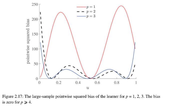
Consider again Example 2.2. The result in (2.53) suggests that \(\mathbb{E} \widehat{\boldsymbol{\beta}} \rightarrow \beta_{p}\) as \(n \rightarrow \infty\), where \(\beta_{p}\) is the solution in the class \(\mathscr{G}_{p}\) given in (2.18). Thus, the large-sample approximation of the pointwise
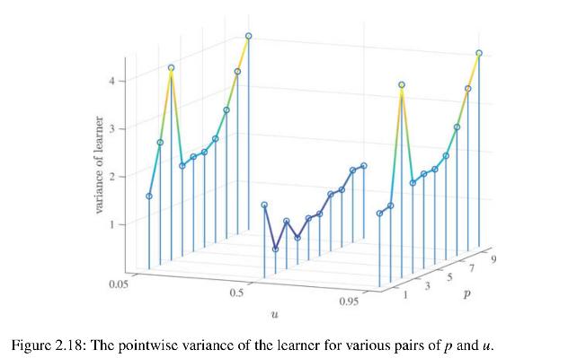
For our running Example 2.2 we can use (2.53) to derive a large-sample approximation of the pointwise variance of the learner \(g_{\mathscr{T}}(\boldsymbol{x})=\boldsymbol{x}^{\top} \widehat{\boldsymbol{\beta}}_{n}\). In particular, show that for large \(n\)\[ \mathbb{V} \operatorname{ar}
Let \(h: \boldsymbol{x} \mapsto \mathbb{R}\) be a convex function and let \(\boldsymbol{X}\) be a random variable. Use the subgradient definition of convexity to prove Jensen's inequality:\[ \begin{equation*} \mathbb{E} h(\boldsymbol{X}) \geqslant h(\mathbb{E} \boldsymbol{X}) \tag{2.56}
Using Jensen's inequality, show that the Kullback-Leibler divergence between probability densities \(f\) and \(g\) is always positive; that is,\[ \mathbb{E} \ln \frac{f(\boldsymbol{X})}{g(\boldsymbol{X})} \geqslant 0 \]where \(\boldsymbol{X} \sim f\).
The purpose of this exercise is to prove the following Vapnik-Chernovenkis bound: for any finite class \(\mathscr{G}\) (containing only a finite number \(|\mathscr{G}|\) of possible functions) and a general bounded loss function, \(l \leqslant\) Loss \(\leqslant u\), the expected statistical error
Consider the problem in Exercise 16a above. Show that\[ \left|\ell_{\mathscr{T}}\left(g_{\mathscr{T}}^{\mathscr{G}}\right)-\ell\left(g^{\mathscr{G}}\right)\right| \leqslant 2 \sup _{g \in
Show that for the normal linear model \(\boldsymbol{Y} \sim \mathscr{N}\left(\mathbf{X} \beta, \sigma^{2} \mathbf{I}_{n}\right)\), the maximum likelihood estimator of \(\sigma^{2}\) is identical to the method of moments estimator (2.37).
Let \(X \sim \operatorname{Gamma}(\alpha, \lambda)\). Show that the pdf of \(Z=1 / X\) is equal to\[ \frac{\lambda^{\alpha}(z)^{-\alpha-1} \mathrm{e}^{-\lambda(z)-1}}{\Gamma(\alpha)}, \quad z>0 \]
Consider the sequence \(w_{0}, w_{1}, \ldots\),where \(w_{0}=g(\boldsymbol{\theta})\) is a non-degenerate initial guess and \(w_{t}(\boldsymbol{\theta}) \propto w_{t-1}(\boldsymbol{\theta}) g(\tau \mid \boldsymbol{\theta}), t>1\). We assume that \(g(\tau \mid \boldsymbol{\theta})\) is not the
Consider the Bayesian model for \(\tau=\left\{x_{1}, \ldots, x_{n}\right\}\) with likelihood \(g(\tau \mid \mu)\) such that \(\left(X_{1}, \ldots, X_{n} \mid \mu\right) \sim_{\text {idd }} \mathscr{N}(\mu, 1)\) and prior pdf \(g(\mu)\) such that \(\mu \sim \mathscr{N}(u, 1)\) for some
Consider again Example 2.8, where we have a normal model with improper prior \(g(\boldsymbol{\theta})\) \(=g\left(\mu, \sigma^{2}\right) \propto 1 / \sigma^{2}\). Show that the prior predictive pdf is an improper density \(g(x) \propto 1\), but that the posterior predictive density is\[ g(x \mid
Showing 4500 - 4600
of 5757
First
39
40
41
42
43
44
45
46
47
48
49
50
51
52
53
Last
Step by Step Answers