New Semester Started Get 50% OFF Study Help! --h --m --s Claim Now

Question Answers

Textbooks

Find textbooks, questions and answers

Oops, something went wrong!

Change your search query and then try again

Result Not Found

Books FREE
Study Help
Tutors
AI Study Planner NEW
Sell Books

Search
Sign In
Register

study help
business
statistical techniques in business

Introduction To Mathematical Statistics 7th Edition Robert V., Joseph W. McKean, Allen T. Craig - Solutions

What is the sufficient statistic for θ if the sample arises from a beta distribution in which α = β = θ > 0?
If X1,X2, . . . , Xn is a random sample from a distribution that has a pdf which is a regular case of the exponential class, show that the pdf of Y1 =Σn1 K(Xi) is of the form fY1 (y1; θ) = R(y1) exp[p(θ)y1 + nq(θ)].
Let Y denote the median and let ‾X denote the mean of a random sample of size n = 2k + 1 from a distribution that is N(μ, σ2). Compute E(Y |‾X = ‾x).
Let X1,X2, . . .,Xn be a random sample from a distribution with pdf f(x; θ) = θ2xe−θx, 0 < x < ∞, where θ > 0.(a) Argue that Y = Σn1 Xi is a complete sufficient statistic for θ.(b) Compute E(1/Y ) and find the function of Y which is the unique MVUE of θ.
Show that Y = |X| is a complete sufficient statistic for θ > 0, where X has the pdf fX(x; θ) = 1/(2θ), for −θ < x < θ, zero elsewhere. Show that Y = |X| and Z = sgn(X) are independent.
Let Y1 < Y2 < · · · < Yn be the order statistics of a random sample from a N(θ, σ2) distribution, where σ2 is fixed but arbitrary. Then ‾Y = ‾X is a complete sufficient statistic for θ. Consider another estimator T of θ, such as T = (Yi + Yn+1−i)/2, for i = 1, 2, . . . ,
Let X1, . . .,Xn be a random sample from a distribution of the continuous type with cdf F(x). Let θ = P(X1 ≤ a) = F(a), where a is known. Show that the proportion n−1#{Xi ≤ a} is the MVUE of θ.
Let X be N(0, θ) and, in the notation of this section, let θ' = 4, θ'' = 9, αa = 0.05, and βa = 0.10. Show that the sequential probability ratio test can be based upon the statistic Σn1 X2i . Determine c0(n) and c1(n).
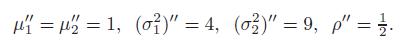
Let X and Y have a joint bivariate normal distribution. An observation (x, y) arises from the joint distribution with parameters equal to eitherorShow that the classification rule involves a second-degree polynomial in x and y. M₁ = ₂ = 0, (0²)' = (0²)' = 1, p' = 1/
Let the random variable X have the pdf f(x; θ) = (1/θ)e−x/θ, 0 < x < ∞, zero elsewhere. Consider the simple hypothesis H0 : θ = θ' = 2 and the alternative hypothesis H1 : θ = θ'' = 4. Let X1,X2 denote a random sample of size 2 from this distribution. Show that the best test of H0
If X1,X2, . . . , Xn is a random sample from a distribution having pdf of the form f(x; θ) = θxθ−1, 0 < x < 1, zero elsewhere, show that a best critical region for testing H0 : θ = 1 against H1 : θ = 2 is C = {(x1, x2, . . . , xn) : c ≤ Пni=1 xi}.
Let X1,X2, . . . , Xn be a random sample from the normal distribution N(θ,1). Show that the likelihood ratio principle for testing H0 : θ = θ' where θ' is specified, against H1 : θ ≠ θ' leads to the inequality |‾x − θ'| ≥ c.(a) Is this a uniformly most powerful test of H0 against
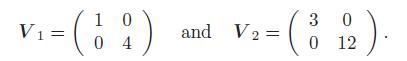
Let W' = (W1,W2) be an observation from one of two bivariate normal distributions, I and II, each with μ1 = μ2 = 0 but with the respective variance covariance matricesHow would you classify W into I or II? 10 V₁ = = (12) 04 V2₂ = and V2 ( 3 0 ₂). 0 12
Let X1,X2, . . . , X10 denote a random sample of size 10 from a Poisson distribution with mean θ. Show that the critical region C defined by Σ101 xi ≥ 3 is a best critical region for testing H0 : θ = 0.1 against H1 : θ = 0.5. Determine, for this test, the significance level α and the power
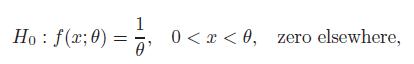
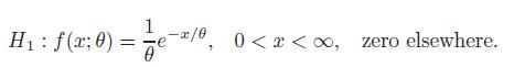
A random sample X1,X2, . . .,Xn arises from a distribution given byorDetermine the likelihood ratio (Λ) test associated with the test of H0 against H1. Ho : f(x;0) = 1/2, 0 < x < 0, zero elsewhere,
Let X1,X2, . . .,Xn be a random sample from a distribution with pdf f(x; θ) = θxθ−1, 0 < x < 1, zero elsewhere, where θ > 0. Show the likelihood has mlr in the statistic Πni=1 Xi. Use this to determine the UMP test for H0 : θ = θ' against H1 : θ < θ', for fixed θ' > 0.
Suppose X1, . . . , Xn is a random sample on X which has a N(μ, σ20) distribution, where σ20 is known. Consider the two-sided hypothesesH0 : μ = 0 versus H1 : μ ≠ 0.Show that the test based on the critical region C = {|‾X| > √σ20/nzα/2} is an unbiased level α test.
Assume that same situation as in the last exercise but consider the test with critical region C∗ = { ‾X > √σ20/nzα}. Show that the test based on C∗ has significance level α but that it is not an unbiased test.
Let X1,X2,X3 be a random sample from the normal distribution N(0,σ2). Are the quadratic forms X21 +3X1X2+X22 +X1X3+X23 and X21−2X1X2 + 2/3X22 − 2X1X2 − X23 independent or dependent?
Compute the mean and variance of a random variable that is χ2(r, θ).
If at least one ϒij ≠ 0, show that the F, which is used to test that each interaction is equal to zero, has non-centrality parameter equal to c Σ=1Σ=11/02.
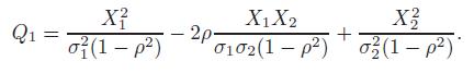
Let X' = [X1,X2] be bivariate normal with matrix of means μ' = [μ1, μ2] and positive definite covariance matrix Σ. LetShow that Q1 is χ2(r, θ) and find r and θ. When and only when does Q1 have a central chi-square distribution? Q₁: X² o²(1 - p²) X1 X2 0102(1-p²) - 2p- + X2/ (1 - p²)
A random sample of size n = 6 from a bivariate normal distribution yields a value of the correlation coefficient of 0.89. Would we accept or reject, at the 5% significance level, the hypothesis that ρ = 0?
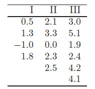
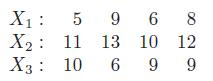
The following are observations associated with independent random samples from three normal distributions having equal variances and respective means μ1, μ2, μ3.Compute the F-statistic that is used to test H0 : μ1 = μ2 = μ3. I II 0.5 2.1 2.1 III 3.0 1.3 3.3 5.1 -1.0 0.0
Compute the mean of a random variable that has a noncentral F-distribution with degrees of freedom r1 and r2 > 2 and non centrality parameter θ.
Extend the Bonferroni procedure described in the last problem to simultaneous testing. That is, suppose we have m hypotheses of interest: H0i versus H1i, i = 1, . . . , m. For testing H0i versus H1i, let Ci,α be a critical region of size α and assume H0i is rejected if Xi ∈ Ci,α, for a sample
Let X1,X2,X3,X4 denote a random sample of size 4 from a distribution which is N(0, σ2). Let Y = Σ41 aiXi, where a1, a2, a3, and a4 are real constants. If Y2 and Q = X1X2 − X3X4 are independent, determine a1, a2, a3, and a4.
Show that the square of a noncentral T random variable is a noncentral F random variable.
Suppose X1, . . . , Xn are independent random variables with the common mean μ but with unequal variances σ2i = Var(Xi).(a) Determine the variance of ‾X.(b) Determine the constant K so that Q = K Σni=1(Xi − ‾X)2 is an unbiased estimate of the variance of ‾X.
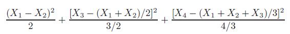
Let X1,X2,X3,X4 be a random sample of size n = 4 from the normal distribution N(0,1). Show that Σ4i=1(Xi − ‾X)2 equalsand argue that these three terms are independent, each with a chi-square distribution with 1 degree of freedom. (X₁X₂)² [X3 - (X₁ + X₂)/2]² [X₁-(X₁ + X2 +
Let A be the real symmetric matrix of a quadratic form Q in the observations of a random sample of size n from a distribution which is N(0, σ2). Given that Q and the mean ‾X of the sample are independent, what can be said of the elements of each row (column) of A?
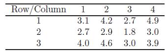
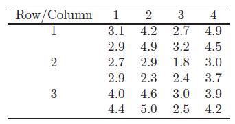
Given the following observations associated with a two-way classification with a = 3 and b = 4, compute the F-statistic used to test the equality of the column means (β1 = β2 = β3 = β4 = 0) and the equality of the row means (α1 = α2 = α3 = 0), respectively. Row/Column 1 2 3 123 2 3 4 3.1 4.2
Let X1 and X2 be two independent random variables. Let X1 and Y = X1+X2 be χ2(r1, θ1) and χ2(r, θ), respectively. Here r1 < r and θ1 ≤ θ. Show that X2 is χ2(r − r1, θ − θ1).
Let μ1, μ2, μ3 be, respectively, the means of three normal distributions with a common but unknown variance σ2. In order to test, at the α = 5% significance level, the hypothesis H0 : μ1 = μ2 = μ3 against all possible alternative hypotheses, we take an independent random sample of size 4
Suppose X1, . . . , Xn are correlated random variables, with common mean μ and variance σ2 but with correlations ρ (all correlations are the same).(a) Determine the variance of ‾X.(b) Determine the constant K so that Q = KΣni=1(Xi − ‾X)2 is an unbiased estimate of the variance of ‾X.
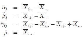
With the background of the two-way classification with c > 1 observations per cell, show that the maximum likelihood estimators of the parameters areShow that these are unbiased estimators of the respective parameters. Compute the variance of each estimator. âi 3₁ Vij û X.
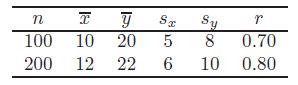
Two experiments gave the following results:Calculate r for the combined sample. n T y 100 10 20 200 12 22 Sx Sy 5 8 6 10 r 0.70 0.80
The driver of a diesel-powered automobile decided to test the quality of three types of diesel fuel sold in the area based on mpg. Test the null hypothesis that the three means are equal using the following data. Make the usual assumptions and take α = 0.05. Brand A: 38.7 39.2 40.1 38.9 Brand B:
Given the following observations in a two-way classification with a = 3, b = 4, and c = 2, compute the F-statistics used to test that all interactions are equal to zero (ϒij = 0), all column means are equal (βj = 0), and all row means are equal (αi = 0), respectively. Row/Column 1 2 3 1 2
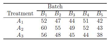
We wish to compare compressive strengths of concrete corresponding to a = 3 different drying methods (treatments). Concrete is mixed in batches that are just large enough to produce three cylinders. Although care is taken to achieve uniformity, we expect some variability among the b = 5 batches
Let Q1 and Q2 be two nonnegative quadratic forms in the observations of a random sample from a distribution which is N(0, σ2). Show that another quadratic form Q is independent of Q1 +Q2 if and only if Q is independent of each of Q1 and Q2.
Show that the covariance between ˆα and ˆβ is zero.
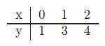
Fit y = a + x to the databy the method of least squares. X y 0 1 1 3 2 4
Suppose X is an n × p matrix with rank p.(a) Show that ker(X'X) = ker(X).(b) Use part (a) and the last exercise to show that if X has full column rank, then X'X is nonsingular.
Fit by the method of least squares the plane z = a + bx + cy to the five points (x, y, z) : (−1,−2, 5), (0,−2, 4), (0, 0, 4), (1, 0, 2), (2, 1, 0).
Suppose Y is an n × 1 random vector, X is an n × p matrix of known constants of rank p, and β is a p × 1 vector of regression coefficients. Let Y have a N(Xβ, σ2I) distribution. Discuss the joint pdf of ˆβ = (X'X)−1 X'Y and Y' [I −X(X' X)−1X' ]Y /σ2.
Let the independent normal random variables Y1, Y2, . . . , Yn have, respectively, the probability density functions N(μ, ϒ2x2i), i = 1, 2, . . ., n, where the given x1, x2, . . . , xn are not all equal and no one of which is zero. Discuss the test of the hypothesis H0 : ϒ = 1, μ unspecified,
Let Y1, Y2, . . . , Yn be n independent normal variables with common unknown variance σ2. Let Yi have mean βxi, i = 1, 2, . . ., n, where x1, x2, . . . , xn are known but not all the same and β is an unknown constant. Find the likelihood ratio test for H0 : β = 0 against all alternatives. Show
Let X be a continuous random variable with pdf f(x). Suppose f(x) is symmetric about a; i.e., f(x − a) = f(−(x − a)). Show that the random variables X − a and −(X − a) have the same pdf.
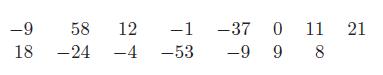
Obtain the sensitivity curves for the sample mean, the sample median and the Hodges–Lehmann estimator for the following data set. Evaluate the curves at the values −300 to 300 in increments of 10 and graph the curves on the same plot. Compare the sensitivity curves. -9 58 12 -1 18 -24 -4
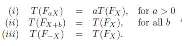
Let X be a random variable with cdf F(x) and let T (F) be a functional. We say that T (F) is a scale functional if it satisfies the three propertiesShow that the following functionals are scale functionals.(a) The standard deviation, T (FX) = (Var(X))1/2.(b) The interquartile range, T (FX) = F−1X
Let ^Fn(x) denote the empirical cdf of the sample X1,X2, . . .,Xn. The distribution of ^Fn(x) puts mass 1/n at each sample item Xi. Show that its mean is ‾X. If T (F) = F−1(1/2) is the median, show that T (^Fn) = Q2, the sample median.
Let X be a continuous random variable with cdf F(x). Suppose Y = X+Δ, where Δ > 0. Show that Y is stochastically larger than X.
Suppose X is a random variable with mean 0 and variance σ2. Recall that the function Fx,ϵ(t) is the cdf of the random variable U = I1−ϵX + [1 − I1−ϵ]W, where X, 1−ϵ, and W are independent random variables, X has cdf FX(t), W has cdf Δx(t), and I1−ϵ has a binomial(1,1 − ϵ )
Suppose that the hypothesis H0 concerns the independence of two random variables X and Y . That is, we wish to test H0 : F(x, y) = F1(x)F2(y), where F, F1, and F2 are the respective joint and marginal distribution functions of the continuous type, against all alternatives. Let (X1, Y1), (X2, Y2), .
Let the scores a(i) be generated by aϕ(i) = ϕ[i/(n+ 1)], for i = 1, . . . , n, where ∫10 ϕ(u) du = 0 and ∫10 ϕ2(u) du = 1. Using Riemann sums, with subintervals of equal length, of the integrals ∫10 ϕ(u) du and ∫10 ϕ2(u) du, show that Σni=1 a(i) ≈ 0 andΣni=1 a2(i) ≈ n.
Suppose the random variable e has cdf F(t). Let ϕ(u) =√12[u − (1/2)],0 < u < 1, denote the Wilcoxon score function.(a) Show that the random variable ϕ[F(ei)] has mean 0 and variance 1.(b) Investigate the mean and variance of ϕ[F(ei)] for any score function ϕ(u) which satisfies ∫10
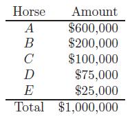
The following amounts are bets on horses A,B,C,D, and E to win.Suppose the track wants to take 20% off the top, namely, $200,000. Determine the payoff for winning with a $2 bet on each of the five horses. (In this exercise, we do not concern ourselves with “place” and “show.”)
Let Y have a binomial distribution in which n = 20 and p = θ. The prior probabilities on θ are P(θ = 0.3) = 2/3 and P(θ = 0.5) = 1/3. If y = 9, what are the posterior probabilities for θ = 0.3 and θ = 0.5?
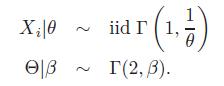
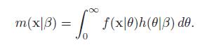
Consider the Bayes modelBy performing the following steps, obtain the empirical Bayes estimate of θ.(a) Obtain the likelihood function(b) Obtain the mle ^β of β for the likelihood m(x|β).(c) Show that the posterior distribution of Θ given x and ^β is a gamma distribution.(d) Assuming
Show that P(C) = 1.
Show that P(Cc) = 1 − P(C).
Let X1,X2, . . . , Xn denote a random sample from a Poisson distribution with mean θ, 0 < θ < ∞. Let Y = Σn1 Xi. Use the loss function L[θ, δ(y)] = [θ−δ(y)]2. Let θ be an observed value of the random variable Θ. If Θ has the prior pdf h(θ) = θα−1e−θ/β/Γ(α)βα, for 0
Show that if C1 ⊂ C2 and C2 ⊂ C1 (that is, C1 ≡ C2), then P(C1) = P(C2).
Show that if C1, C2, and C3 are mutually exclusive, then P(C1∪C2∪C3) = P(C1) + P(C2) + P(C3).
Show that P(C1 ∪ C2) = P(C1) + P(C2) − P(C1 ∩ C2).
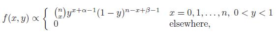
Consider the following mixed discrete-continuous pdf for a random vector (X, Y), (discussed in Casella and George, 1992):for α > 0 and β > 0.(a) Show that this function is indeed a joint, mixed discrete-continuous pdf by finding the proper constant of proportionality.(b) Determine the
If computation facilities are available, write a program for the Gibbs sampler of Exercise 11.4.7. Run your program for α = 10, β = 4, m = 3000, and n = 6000. Obtain estimates (and confidence intervals) of E(X) and E(Y) and compare them with the true parameters.Exercise 11.4.7Consider the
Let Y4 be the largest order statistic of a sample of size n = 4 from a distribution with uniform pdf f(x; θ) = 1/θ, 0 < x < θ, zero elsewhere. If the prior pdf of the parameter g(θ) = 2/θ3, 1 < θ < ∞, zero elsewhere, find the Bayesian estimator δ(Y4) of θ, based upon the
Calculate the lim and ¯lim of each of the following sequences:(a) For n = 1, 2, . . ., an = (−1)n (2 − 4/2n).(b) For n = 1, 2, . . ., an = ncos(πn/2).(c) For n = 1, 2, . . ., an = 1/n + cos πn/2 + (−1)n.
Let {an} and {dn} be sequences of real numbers. Show that lim (an + dn) lim an + lim dn. n→∞ n→∞ n→∞
Let {an} be a sequence of real numbers. Suppose {ank} is a subsequence of {an}. If {ank} → a0 as k→∞, show that limn→∞ an ≤ a0 ≤ ¯limn→∞ an.
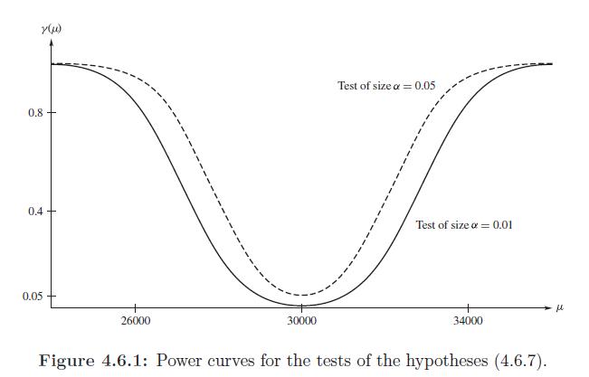
For the test at level 0.05 of the hypotheses given by (4.6.1) with μ0 = 30,000 and n = 20, obtain the power function, (use σ = 5000). Evaluate the power function for the following values: μ = 25,000; 27,500; 30,000; 32,500; and 35,000. Then sketch this power function and see if it agrees with
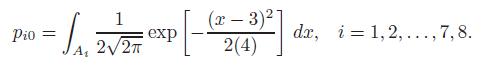
Define the sets A1 = {x : −∞ < x ≤ 0}, Ai = {x : i − 2 < x ≤ i − 1}, i = 2, . . . , 7, and A8 = {x : 6 < x < ∞}. A certain hypothesis assigns probabilities pi0 to these sets Ai in accordance withThis hypothesis (concerning the multinomial pdf with k = 8) is to be tested,
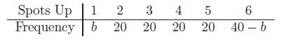
A die was cast n = 120 independent times and the following data resulted:If we use a chi-square test, for what values of b would the hypothesis that the die is unbiased be rejected at the 0.025 significance level? Spots Up 1 2 Frequency b 3 20 20 20 4 4 5 20 6 40-b
A number is to be selected from the interval {x : 0 < x < 2} by a random process. Let Ai = {x : (i − 1)/2 < x ≤ i/2}, i = 1, 2, 3, and let A4 = {x :3/2 < x < 2}. For i = 1, 2, 3, 4, suppose a certain hypothesis assigns probabilities pi0 to these sets in accordance with pi0 =
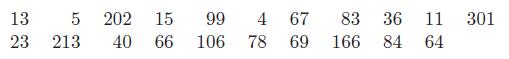
Consider the sample of data:(a) Obtain the five-number summary of these data.(b) Determine if there are any outliers.(c) Boxplot the data. Comment on the plot. 13 5 202 15 99 4 67 83 36 11 301 23 213 40 66 106 78 69 166 84 64
Let Y2 and Yn−1 denote the second and the (n − 1)st order statistics of a random sample of size n from a distribution of the continuous type having a distribution function F(x). Compute P[F(Yn−1) − F(Y2) ≥ p], where 0 < p < 1.
Suppose X is a random variable with the pdf fX(x) = b−1f((x − a)/b), where b > 0. Suppose we can generate observations from f(z). Explain how we can generate observations from fX(x).
Let Y1 < Y2 < · · · < Yn be the order statistics of a random sample of size n from a distribution of the continuous type having distribution function F(x).(a) What is the distribution of U = 1− F(Yj)?(b) Determine the distribution of V = F(Yn) − F(Yj) + F(Yi) − F(Y1), where i <
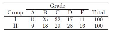
Two different teaching procedures were used on two different groups of students. Each group contained 100 students of about the same ability. At the end of the term, an evaluating team assigned a letter grade to each student. The results were tabulated as follows.If we consider these data to be
Consider the problem from genetics of crossing two types of peas. The Mendelian theory states that the probabilities of the classifications (a) Round and yellow, (b) Wrinkled and yellow, (c) Round and green,(d) Wrinkled and green are 9/16 , 3/16 , 3/16, and 1/16 , respectively. If,
Let Y1 < Y2 < · · · < Y10 be the order statistics of a random sample from a continuous-type distribution with distribution function F(x). What is the joint distribution of V1 = F(Y4) − F(Y2) and V2 = F(Y10) − F(Y6)?
Assume that the weight of cereal in a “10-ounce box” is N(μ, σ2). To test H0 : μ = 10.1 against H1 : μ > 10.1, we take a random sample of size n = 16 and observe that ¯x = 10.4 and s = 0.4.(a) Do we accept or reject H0 at the 5% significance level?(b) What is the approximate p-value of
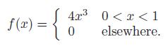
Determine a method to generate random observations for the following pdf:If access is available, write an R function which returns a random sample of observations from this pdf. f(x) = { 42³ 0 0
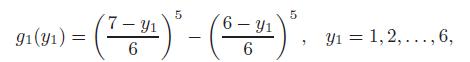
Let f(x) = 1/6, x = 1, 2, 3, 4, 5, 6, zero elsewhere, be the pmf of a distribution of the discrete type. Show that the pmf of the smallest observation of a random sample of size 5 from this distribution iszero elsewhere. 91(y₁) = 7-91 6 CT 5 6-91 6 CT y₁ = 1,2,..., 6,
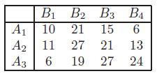
Let the result of a random experiment be classified as one of the mutually exclusive and exhaustive ways A1,A2,A3 and also as one of the mutually exclusive and exhaustive ways B1,B2,B3,B4. Two hundred independent trials of the experiment result in the following data:Test, at the 0.05 significance
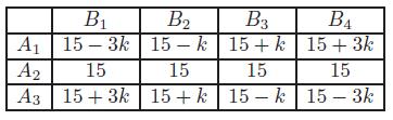
Let the result of a random experiment be classified as one of the mutually exclusive and exhaustive ways A1,A2,A3 and also as one of the mutually exhaustive ways B1,B2,B3,B4. Say that 180 independent trials of the experiment result in the following frequencies:where k is one of the integers 0, 1,
Each of 51 golfers hit three golf balls of brand X and three golf balls of brand Y in a random order. Let Xi and Yi equal the averages of the distances traveled by the brand X and brand Y golf balls hit by the ith golfer, i = 1, 2, . . . , 51. Let Wi = Xi − Yi, i = 1, 2, . . . , 51. Test H0 : μW
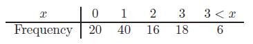
It is proposed to fit the Poisson distribution to the following data:(a) Compute the corresponding chi-square goodness-of-fit statistic.(b) How many degrees of freedom are associated with this chi-square?(c) Do these data result in the rejection of the Poisson model at the α = 0.05 significance
A certain genetic model suggests that the probabilities of a particular trinomial distribution are, respectively, p1 = p2, p2 = 2p(1−p), and p3 = (1−p)2, where 0 < p < 1. If X1,X2,X3 represent the respective frequencies in n independent trials, explain how we could check on the adequacy
Let us say the life of a tire in miles, say X, is normally distributed with mean θ and standard deviation 5000. Past experience indicates that θ = 30,000. The manufacturer claims that the tires made by a new process have mean θ > 30,000. It is possible that θ = 35,000. Check his claim by
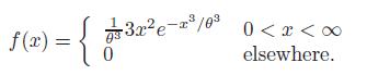
Suppose we are interested in a particular Weibull distribution with pdfDetermine a method to generate random observations from this Weibull distribution. If access is available, write an R function which returns a random sample of observation from a Weibull distribution. f(x)= :{ = 0 3²e-³/0³ 0
Let Y1 < Y2 < · · · < Yn be the order statistics of a random sample of size n from a distribution with pdf f(x) = 1, 0 < x < 1, zero elsewhere. Show that the kth order statistic Yk has a beta pdf with parameters α = k and β = n − k + 1.
Let z∗ be drawn at random from the discrete distribution which has mass n−1 at each point zi = xi − ¯x + μ0, where (x1, x2, . . . , xn) is the realization of a random sample. Determine E(z∗) and V (z∗).
Let Y be b(300, p). If the observed value of Y is y = 75, find an approximate 90% confidence interval for p.
Suppose a random sample of size 2 is obtained from a distribution that has pdf f(x) = 2(1 − x), 0 < x < 1, zero elsewhere. Compute the probability that one sample observation is at least twice as large as the other.
Let Y1 < Y2 be the order statistics of a random sample of size 2 from a distribution of the continuous type which has pdf f(x) such that f(x) > 0, provided that x ≥ 0, and f(x) = 0 elsewhere. Show that the independence of Z1 = Y1 and Z2 = Y2 − Y1 characterizes the gamma pdf f(x), which
It is known that a random variable X has a Poisson distribution with parameter μ. A sample of 200 observations from this distribution has a mean equal to 3.4. Construct an approximate 90% confidence interval for μ.
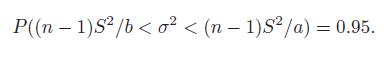
Let X1,X2, . . .,Xn be a random sample from N(μ, σ2), where both parameters μ and σ2 are unknown. A confidence interval for σ2 can be found as follows. We know that (n − 1)S2/σ2 is a random variable with a χ2(n − 1) distribution. Thus we can find constants a and b so that P((n −

Showing 5100 - 5200 of 5757

First
44
45
46
47
48
49
50
51
52
53
54
55
56
57
58

Step by Step Answers

Services

Sitemap
Fun
Definitions
Become Tutor
Used Textbooks
Study Help Categories
Recent Questions
Expert Questions
Campus Wear
Sell Your Books

Company Info

Security
Copyrights
Privacy Policy
Terms & Conditions
SolutionInn Fee
Scholarship
Online Quiz
Give Feedback, Get Rewards

Get In Touch

About Us
Contact Us
Career
Jobs
FAQ
Student Discount
Campus Ambassador

Secure Payment

Download Our App

© 2026 SolutionInn. All Rights Reserved