a. Example 17-2: Mean Conversion, Xseg, Calculations in a Real Reactor Wolfram and Python 1. How do
Question:
a. Example 17-2: Mean Conversion, Xseg, Calculations in a Real Reactor
Wolfram and Python
1. How do CA0, n and k affect the trajectories in X for the segregation model and the LFR?
2. Write a set of conclusions based on your experiments in (i).
Polymath
1. How does the conversion predicted from the segregation model, Xseg, compare with the conversion predicted by the CSTR, PFR, and LFR models for the same mean residence time, tm?
Example 17-2
Calculate the mean conversion in the reactor we have characterized by RTD measurements in Examples 16-1 and 16-2 for a first-order, liquid-phase, irreversible reaction in a completely segregated fluid: A → products The specific reaction rate is 0.1 min–1 at 320 K.
Examples 16-1
Examples 16-2
b. Example 17-3: Mean Conversion for Second-Order Reaction in a Laminar-Flow Reactor Wolfram and Python
1. For what value of k are X and X¯ the farthest apart? Closest together?
2. Vary n and describe what you find with regard to Xseg.
3. Explain how the E-curve varies with n, CA0, and k.
4. Vary n, τ, CA0, and k and describe what you find.
5. Write a set of conclusions for your experiments (i) through (iv).
Polymath
1. (1) Vary k by a factor of 5–10 or so above and below the nominal value given in the problem statement of 4.93 × 10⁻³ dm3/mol/s. When do XPFR and XLFR come close together and when do they become farther apart?
Example 17-3
The liquid-phase reaction between cytidine and acetic anhydride is carried out isothermally in an inert solution of N-methyl-2-pyrrolidone (NMP) with ΘNMP = 28.9. The reaction follows an elementary rate law. The feed is equal molar in A and B with CA0 = 0.75 mol/dm3, a volumetric flow rate of 0.1 dm3/s, and a reactor volume of 100 dm3. Calculate the conversion in (a) an ideal PFR, (b) a BR, and (c) an LFR.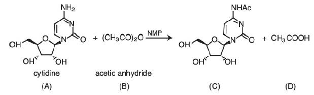
The product (A) cytidine is a cyclopentane with the first carbon position replaced by an oxygen atom. The third and fourth carbon position of cyclopentane is bonded to a hydroxide. The second and fifth carbon position of cyclopentane is hatched bonded to nitrogen and a hydroxide respectively. The nitrogen atom bonded to a cyclopentane occupies the fourth carbon position of the benzene ring. Another nitrogen atom is replaced in the second carbon position of benzene. The first and third carbon position of the benzene is single and double-bonded to ammonia and an oxygen atom respectively. The cytidine combines with the product (B) acetic anhydride (CH3CO)2O that reacts in the presence of NMP to form product (C), the same as the structure of cytidine, but the ammonia is replaced by NHAc molecule and product
(D) CH3COOH.
A + B → C + D
Additional information: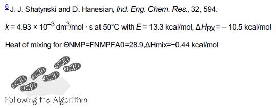
c. Example 17-4: Conversion Bounds for a Nonideal Reactor
Wolfram and Python
1. For what value of k are X and X¯ the farthest apart? Closest together?
2. Vary n and describe what you find with regard to Xseg.
3. Explain how the E-curve varies with n, CA0, and k.
4. Vary n, τ, CA0, and k and describe what you find.
5. Write a set of conclusions for your experiments (i) through (iv).
Polymath
1.
(1) Vary the parameter kCA0, whose nominal value is
kCA0=(0.01 dm3mol⋅s)(8 moldm3)=0.08/s
by a factor of 10 above and below the value nominal of 0.08 s–1 and describe when Xseg and Xmm come closer together and when they become farther apart.
(2) How do Xmm and Xseg compare with XPFR, XCSTR, and XLFR for the same mean residence time?
(3) How would your results change if T = 350 K with E = 10 kcal/mol? How would your answer change if the reaction was pseudo first order with kCA0 = 4 × 10⁻³/s?
Example 17-4
The liquid-phase, second-order dimerization 2A→BrA=−kCA2 for which k = 0.01 dm3/mol·min is carried out at a reaction temperature of 320 K. The feed is pure A with CA0 = 8 mol/dm3. The reactor is nonideal. The reactor volume is 1000 dm3, and the feed rate for our dimerization is We wish to know the bounds on the conversion for different possible degrees of micromixing for the RTD of this reactor. What are these bounds?
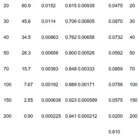
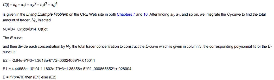
The Jofostan students carried out a tracer test by throwing 100 g of tracer (N0 = 100 g) into the reactor that had an entering volumetric flow rate of 25 dm3/min (υ0 = 25 dm3/min) and then measured the exit concentration (C(t) as a function of time t) and the results are shown in columns 1 and 2 of Table E17-4.1. The exit concentration, that is, the C-curve, was then fit to a polynomial. A tutorial on how to fit the tracer data points to a polynomial, for example,
Table E17-4.1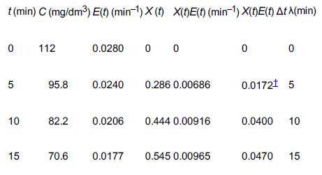
d. Example 17-5: Using Software to Make Maximum Mixedness Model Calculations
Wolfram and Python
1. Individually vary k, CA0 and n and describe how the profile X as a function of Z changes.
2. Individually vary k, CA0 and n and describe how the rate –rA changes as you vary k, CA0 and n.
3. Write a set of conclusions.
Polymath
1.
(1) Vary the parameters kCA0, above and below the nominal value 0.08 s–1, by a factor of 10 and describe when Xmm and Xseg come closer together and when they become farther apart.
(2) How do Xmm and Xseg compare with XPFR, XCSTR, and XLFR for the same tm?
(3) How would your results change if the reaction was pseudo first order with k1 = CA0k = 0.08 min–1?
(4) If the reaction was third order with kCA02=0.08 min−1?
(5) If the reaction was half order with kCA01/2=0.08 min−1? Describe any trends.
Example 17-5
Use an ODE solver to determine the conversion predicted by the maximum mixedness model for the E(t) curve given in Example E17-4.
e. Example 17-6a: RTD and Complex Reaction for an Asymmetric RTD (shown on the CRE Web site at http://www.umich.edu/~elements/6e/17chap/live.html)
Wolfram and Python
1. Vary k1, k2, and k3 and describe how the conversion changes.
2. Vary k1, k2, and k3 and describe how the concentration and selectivity change.
3. Vary k1, k2, and k3 and describe how the rate changes.
4. Write a set of conclusions.
Polymath
1. Download the Living Example Problem from the CRE Web site.
If the activation energies in cal/mol are E1 = 5000, E2 = 1000, and E3 = 9000, how would the selectivities and conversion of A change as the temperature was raised or lowered around 350 K?
Example 17-6a
Consider the following set of liquid-phase reactions A+B→k1CA→k2DB+D→k3E
which are occurring in two different reactors with the same mean residence time, tm = 1.26 minutes. However, the RTD is very different for each of the reactors, as can be seen in Figures E17-6.1 and E17-6.2.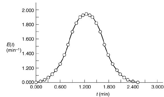
A graph shows an asymmetric distribution. The horizontal axis represents t (minutes) ranging from 0.000 to 3.000, in increments of 0.600. The vertical axis represents E of t (minutes inverse) ranging from 0.000 to 2.000 with the kink present between range 0.000 to 1.200. The bell curve is drawn touching the horizontal axis that starts from the point (0.000, 0.000) and ends at the point (2.500, 0.000) with its peak at point (1.400, 1.900). Note: All points are marked approximately. Two different reactors with different RTDs, but the same mean residence time tmA graph shows a bimodal distribution. The horizontal axis represents t (minutes) ranging from 0.000 to 6.000, in increments of 1.200. The vertical axis represents E of t
(minutes inverse) ranging from 0.000 to 0.800, in increments of 0.160. A curve starts from the point (0.000, 0.170), increases gradually to 0.640, fluctuates and
decreases to the point (6.000, 0.000). Note: All points are marked approximately.
1. Fit polynomials to the RTDs for each reactor.
2. Determine the product distribution and selectivities (e.g., ŜC/D, ŜD/E) for
1. The segregation model.
2. The maximum mixedness model.
Before carrying out any calculations, what do you think the exit concentrations and conversion will be for these two very different RTDs with the same mean residence
time?
Additional information: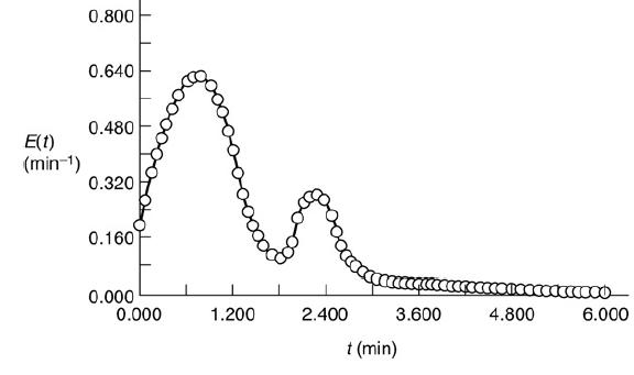
A graph shows a bimodal distribution. The horizontal axis represents t (minutes) ranging from 0.000 to 6.000, in increments of 1.200. The vertical axis represents E of t (minutes inverse) ranging from 0.000 to 0.800, in increments of 0.160. A curve starts from the point (0.000, 0.170), increases gradually to 0.640, fluctuates and decreases to the point (6.000, 0.000). Note: All points are marked approximately.
1. Fit polynomials to the RTDs for each reactor.
2. Determine the product distribution and selectivities (e.g., ŜC/D, ŜD/E) for
1. The segregation model.
2. The maximum mixedness model. Before carrying out any calculations, what do you think the exit concentrations and conversion will be for these two very different RTDs with the same mean residence
time?
Additional information:![]()
f. Example 17-6b: RTD and Complex Reaction with a Bimodal RTD (shown on the CRE Web site at http://www.umich.edu/~elements/6e/17chap/live.html)
Wolfram and Python
1. Vary k1, k2, and k3 and describe how the conversion changes.
2. Vary k1, k2, and k3 and describe how the concentration and selectivity change.
3. Vary k1, k2, and k3 and describe how the rate changes.
4. Write a set of conclusions.
Step by Step Answer:
a i Increase in k increases X for both segregation model as well as LFR increase in n decreases X for both segregation model as well as LFR whereas change in Cao has no effect on both ii 1 Observe tha...View the full answer