

Question: a. Example 18-1. Concentration and Conversion Profiles for Dispersion and Reaction in a Tubular Reactor Wolfram and Python 1. Vary Pclet number, Per from its
a. Example 18-1. Concentration and Conversion Profiles for Dispersion and Reaction in a Tubular Reactor
Wolfram and Python
1. Vary Péclet number, Per from its largest to smallest value. Describe how the outlet concentration for “reaction with dispersion” deviates from that of “Ideal
PFR” as Per is varied.
2. What should be the minimum value of space time, τ, at which conversion reaches at least 95% for reaction with dispersion.
3. If the reaction rate constant is increased to 0.5 min–1, what should be the value of Péclet number, Per, so as to achieve conversion of 90%.
4. Vary the sliders and write a set of conclusions.
Example 18-1
A first-order reaction with k = 0.25 min–1 is occurring in a tubular reactor with dispersion where the space time is τ = 5.15 min and the Péclet number is Per = 7.5. In Example 18-2, we will show how to use this tracer data to calculate the Damköler number and Péclet number. Plot the concentration and conversion profiles for a closed-closed system.
b. Example 18-2. Comparing Conversion Using Dispersion, PFR, CSTR, and Tanks-in-Series Models for Isothermal Reactors
Wolfram and Python
1. Which parameter will you vary so that conversion obtained by dispersion model approaches to conversion obtained using ideal PFR model.
2. What is the number of tanks in series required so that conversion obtained by the tank-in-series model is more than conversion obtained by the dispersion model?
3. Write a set of conclusions after you have varied all the parameter values.
Example 18-2
The first-order reaction A → B
is carried out in a 10-cm-diameter tubular reactor 6.36 m in length. The specific reaction rate is 0.25 min–1. The results of a tracer test carried out on this reactor are shown in Table E18-2.1.
TABLE E18-2.1 EFFLUENT TRACER CONCENTRATION AS A FUNCTION OF TIME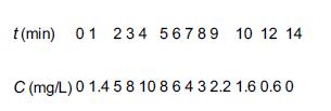
Calculate the conversion using (a) the closed vessel dispersion model, (b) PFR, (c) the tanks-in-series model, and (d) a single CSTR.
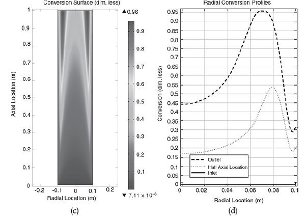
c. Example 18-3. Isothermal Reaction with Radial and Axial Dispersion in an LFR
Go to the COMSOL link LEP 18-3 in Chapter 18 on the CRE Web site.
1. Vary the velocity and describe how the radial concentration profiles as well as the surface plot changes.
2. Vary the reactor radius and describe what you find.
3. Vary DAB and describe how the radial concentration profiles and the exit concentration change.
4. Compare the radial concentration profiles at the inlet, exit, and halfway down the reactor with the radially averaged axial concentration when you vary DAB
and U and describe what you find.
5. What combination of parameters, for example, (Da/UL) do not significantly change the base case profile when varied over a wide range? For example,
diameter is between 0.01 dm and 1 m and the velocity varies from U = 0.01 cm/s to 1 m/s with DAB = 10–5 cm2/s with υ = μ/ρ = 0.01 m2/s. Is there a diameter that minimizes or maximizes your conversion?
6. To what parameters or groups of parameters (e.g., kL2/Da) would the conversion be most sensitive? What if the first-order reaction were carried out in tubular reactors of different diameters, but with the space time, τ, remaining constant? The diameters would range from a diameter of 0.1 dm to a diameter of 1 m for a kinematic viscosity υ = μ/ρ = 0.01 cm2/s, U = 0.1 cm/s, and DAB = 10–5 cm2/s. How would your conversion change? Is there a diameter that would maximize or minimize conversion in this range?
7. Which type of velocity profile gives the higher outlet concentration?
8. What two parameters would reduce the radial variation in concentration?
9. Which variable has very little effect on radial variation in concentration?
10. What is the effect of diffusivity on the outlet concentration?
11. Keep Da and L/R constant and vary the reaction order n, (0.5 ≤ n ≤ 5) for different Péclet numbers. Are there any combinations of n and Pe where dispersion is more important or less important on the exit concentration? What generalizations can you make? Hint: for n 12. Write a set of conclusions based on your experiments (i) through (xi).
Example 18-3
We now consider flow, reaction and dispersion in cylindrical pipes. The parameter values (e.g., k, U0) will be varied using a COMSOL program. Initially we will use the following values, k = 8.33 × 10⁻⁶ m3/mol · s, CA0 = 500 mol/m3, U0 = 0.021 m/s, and DA0 = 1.25 × 10⁻⁶ m2/s.
1. Plot the concentration surface for to and ϕ = 0 to ϕ = 1 and λ = 0 to λ = 1. To make this plot, go to the CRE Web site and load the COMSOL LEP instruction on How to Access COMSOL (http://www.umich.edu/~elements/6e/comsol/comsol_access_instructions.html). Vary the parameters and run the simulation.
2. Plot the radial concentration profile.
3. Plot the axial profiles at ϕ = 0 and ϕ = 1/2.
4. Plot the radially averaged axial concentration profiles CA(z) (i.e., ϕ(λ)).
d. Example 18-4. Tubular Reactor with Axial and Radial Temperature and Concentration Gradients
Use the COMSOL LEP on the Web site to explore radial effects in a tubular reactor. The Additional Material on the Web site describes this LEP in detail
(http://umich.edu/~elements/6e/18chap/expanded_ch18_radial.pdf). Tutorials on how to access and use COMSOL can be found at
(http://umich.edu/~elements/6e/software/software_comsol.html).
1. Vary the heat transfer coefficient, U, and observe the effect on both the conversion and temperature profiles. Why is there an effect of U on the profiles at
low values of U, but not at higher values of U?
2. What is the effect of the different diffusivities, Da, on the conversion? Should Da be minimized or maximized?
3. What parameter would you vary so that the maximum of the radial conversion profile becomes 1? What is the value of that parameter?
4. How would your profiles change if the velocity profile was changed to plug flow (U = U0)? Based on your observations, which of the two profiles, namely, laminar flow and plug flow, would you recommend for a larger conversion? How does the change in velocity profile make an effect in the temperature profile?
5. Intuitively, how do you expect the radial conversion to vary with diffusion coefficient? Explain the reason behind your intuition. Verify this by varying the diffusion coefficient. Investigate axial and radial conversion and write two conclusions.
Example 18-4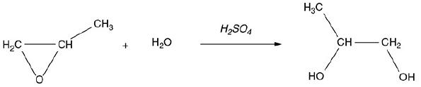
The liquid phase reaction was analyzed using COMSOL to study both axial and radial variations, and the details can be found on the home page of the CRE Web site, www.umich.edu/~elements/6e/index.html, by clicking on the Additional Material for Chapter 18. The algorithm for this example can be found on the Web site: (http://umich.edu/~elements/6e/18chap/expanded_ch18_radial.pdf). Web Figure E12-8.1 is a screen shot from COMSOL of the base case reactor and reaction parameters. In the COMSOL LEP you are asked “What if…” questions about varying the base case parameters. Typical radial (a) and axial (b) temperature profiles for this example are shown in Figure E18-4.1.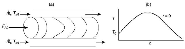
Radial (a) and axial (b) temperature profiles. Figure (a) shows the radial temperature profile. It shows the flow and reaction in a tubular reactor at the entrance and exit of the reactor. The flow rate at the entrance is marked as F subscript A0. The direction of flow rate and of Radial location times temperature is given from left to right. The graph in figure b shows a normal distribution curve for axial temperature profile drawn between temperature and height of the particle, z. The curve starts at a point, T0 on the y-axis, increases to a maximum point and decreases gradually. The graphical solutions to the COMSOL code are shown in Figure E18-4.2. Results of the COMSOL simulation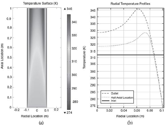
e. Example 18-5. Using a Tracer to Determine the Model Parameters in a CSTR with Dead Volume and Bypass Model
Wolfram and Python
1. For the case of no dead volume (α = 1), vary bypass volume fraction, β, and describe its effect on outlet concentration.
2. Repeat part (i) for the case of no bypass volume (β = 0) and vary = to observe its effect on outlet concentration.
3. From your observation in part (i) and part (ii), which of the two model parameters (α or β) have more impact on outlet concentration and conversion?
Explain.
4. Write a set of conclusions based on your experiments in (i) through (iii).
Example 18-5
The following tracer concentration time data was obtained from a step input to the system in Figure 18-14.
TABLE E18-5.1 TRACER DATA FOR STEP INPUT
CT (mg/dm3) 1000 1333 1500 1666 1750 1800
t (min) 4 8 10 14 16 18
The entering tracer concentration is CT0 = 2000 mg/dm3.
1. Determine the model parameters α and β where α = Vs/V and β = υb/υ0.
2. Determine the conversion for a second-order reaction with CA0 = 2 kmol/m3, τ = 10 min, and k = 0.28 m3/kmol · min.
Figure 18-14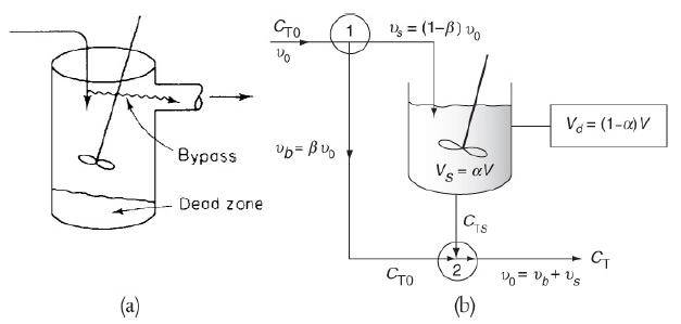
f. Example 18-6. CSTR with Interchange
Wolfram and Python
1. For a fixed value of α (say α = 0.5), how does the conversion vary with increase in β? Explain.
2. Vary α and describe its impact on the exit concentration.
3. Vary rate constant, k, and describe what you find about its effect on exit concentration.
4. Write a set of conclusions based on your experiments in (i) through (iii).
Example 18-6
A pulse trace test was carried out on the model system shown in Figure 18-15 (http://www.umich.edu/~elements/6e/18chap/Ch18_Web-Additional%20Material.pdf) with CT0=2000 mg/dm3 and τ=Vυ0=1000 dm325 dm3/ min=40min, and the results are shown in Table E18-6.1.
TABLE E18-6.1 TRACER DATA FOR PULSE INPUT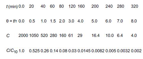
1. Find the interchange parameters α and β.
2. Find the conversion for a first-order reaction with k = 0.03 min–1.
3. Find the corresponding conversion in an ideal CSTR and in an ideal PFR.
Figure 18-15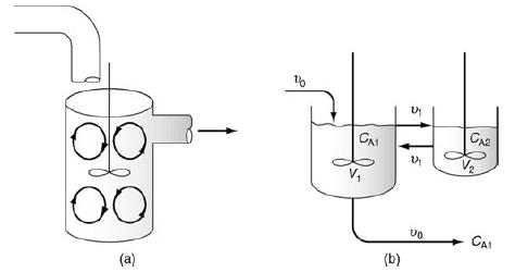
t(min) 01 234 56789 10 12 14 C (mg/L) 0 1.45 8 10 8 6 4 3 2.2 1.6 0.6 0
Step by Step Solution
3.36 Rating (152 Votes )
There are 3 Steps involved in it
a i As Peclet number is varied from its largest to smallest value outlet concentration for reaction with dispersion deviates more from Ideal PFR case ii At space time 16min conversion reaches 95 for r... View full answer

Get step-by-step solutions from verified subject matter experts