Estimating cost and production functions for industrial plants is important. Decisions are based on estimated average and marginal cost, and average and marginal products. Suppose a manufacturing plant for a particular firm has output modeled as \(Q=\beta_{1}+\beta_{2} M G T \_E F F+\beta_{3} C A P+\beta_{4} L A B+e\), where \(Q\) is the output in a particular manufacturing plant, \(M G T_{-} E F F\) is a managerial efficiency index, \(C A P\) is capital stock input index and \(L A B\) is labor input index.

a. What is the interpretation of \(\beta_{2}\) ? What sign should it have?

b. Measuring \(M G T_{-} E F F\) is difficult. Suppose we propose to estimate the model

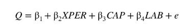
where XPER is the plant manager's experience, measured in years. What should the sign of \(\beta_{2}\) be now? Why might we worry that XPER is endogenous? 

c. We use data from 75 plants to estimate the model in (b). The least squares estimates are

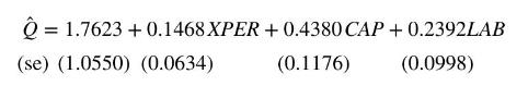
Are the signs of the coefficients and their significance consistent with your expectations? Explain.

d. If XPER is endogenous, what is the direction of the bias of the OLS estimator? Explain. [Hint: Remember your answer to part (b).]

e. Suppose we consider \(A G E\), the age of the plant manager, as an instrument. Does it satisfy the criteria for an IV based on your economic reasoning? Why or why not?

f. In the OLS regression of XPER on CAP, \(L A B\), and \(A G E\), the \(t\)-value for the coefficient of \(A G E\) is 3.13. What information does this provide us about the feasibility of carrying out IV/2SLS?
g. We add the residuals from part (f) to the model in (b) to obtain

The \(t\)-statistic for the null hypothesis \(H_{0}: \beta_{5}=0\) from this regression is -2.2 . What should we infer from it?
h. The two-stage least squares estimates are

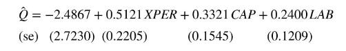
What are the differences in these estimates versus the OLS estimates? Are the differences consistent with your expectations, relative to the OLS estimates? Explain.
i. Reasoning that \(A G E\) is an adequate IV, a staff economist decides to add \(A G E \times L A B\) and \(A G E \times\) \(C A P\) as IV also. Are these likely to be valid IV and uncorrelated with the regression error term? To test this, the two-stage least squares residuals are regressed on CAP, \(L A B, A G E, A G E \times L A B\), and \(A G E \times C A P\). The resulting \(R^{2}\) is 0.0045 . What do you think about the validity of the IV now?
j. The economist regresses XPER on \(C A P, L A B, A G E, A G E \times L A B\), and \(A G E \times C A P\). The \(F\)-test of the joint significance of \(A G E, A G E \times L A B\), and \(A G E \times C A P\) is 3.3. Do you think it is advisable to use the interaction variables as IV in the estimation? Justify your answer.

Transcribed Image Text:

Q = B+ BXPER + 3 CAP + LAB + e