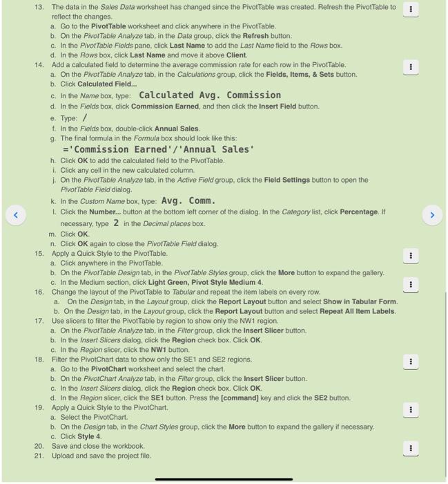
13. The data in the Sales Data worksheet has changed since the PivotTable was created. Retresh the PivotTable to rellect the changes. a. Go to the PivotTable worksheet and click anywhere in the PivorTable. b. On the Pivot Table Analyze tab, in the Data group, click the Refresh button. c. In the PivotTable Fields pane, click Last Name to add the Last Name field to the Rows box. d. In the Rows box, click Last Name and move it above Client. 14. Add a calculated field to determine the average commission rate for each row in the PivotTable. a. On the PivotTable Analyze tab, in the Calculations group, click the Fields, Items, \& Sets button. b. Click Calculated Field... c. In the Name box, type: Calculated Avg. Commission d. In the Fields box, click Commission Earned, and then click the Insert Field button. e. Type: / t. In the Fields box, double-click Annual Sales. 9. The final formula in the Formula box should look like this: =' Commission Earned '/'Annual Sales' h. Click OK to add the calculated field to the PivotTable. 1. Click any cell in the new calculated column. 1. On the PivotTable Analyze tab, in the Active Field group, click the Field Settings button to open the PivotTable Fleld dialog. k. In the Custom Name box, type: Avg. Comm. L. Click the Number... button at the bottom left comer of the dialog. In the Catogory list, click Percentage. If necessary, type 2 in the Decimal places box. m. Click OK. n. Click OK again to close the PivorTable Field dialog. 15. Apply a Quick Style to the PivotTable. a. Click anywhere in the PivotTable. b. On the PivotTable Design tab, in the PivotTable Styles group, click the More button to expand the gallery. c. In the Medium section, click Light Green, Pivot Style Medium 4. 16. Change the layout of the PivotTable to Tabular and repeat the item labels on every row. a. On the Design tab, in the Layout group, click the Report Layout button and select Show in Tabular Form. b. On the Design tab, in the Layout group, click the Report Layout button and select Repeat All Item Labels. 17. Use slicers to filter the PlvotTable by region to show only the NW1 region. a. On the PivotTable Analyze tab, in the Filter group, click the Insert Slicer button. b. In the Insert Slicers dialog, click the Region check box, Click OK. c. In the Region slicer, click the NW1 button. 18. Filter the PivotChart data to show only the SE1 and SE2 regions. a. Go to the Pivotchart worksheet and select the chart. b. On the PivotChart Analyze tab, in the Filter group, click the Insert Slicer button. c. In the Insert Slicers dialog, click the Region check box. Click OK. d. In the Region slicer, click the SE1 button. Press the [command] key and click the SE2 button. 19. Apply a Quick Style to the PivotChart. a. Select the PivotChart. b. On the Design tab, in the Chart Styles group, click the More button to expand the gallery if necessary. c. Click Style 4. 20. Save and close the workbook. 21. Upload and save the project file