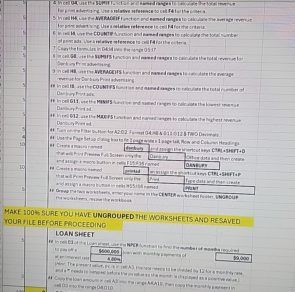
$4$ In cellG$4,$ use the SUMIF function and named ranges to calculate the total revenue forprint advertising. Use a relative reference to cell F$4$ for the criteria.

$5$ In cell $H4,$ use the AVERAGEIF function and named range s to calculate the average revenue for print advertising. Use a relative refere nce to cell F$4$ for the criteria.

$6$ In cell I$4,$ use the COUNTIF function and named ranges to calculate the total number of print ads. Use a relative reference to cell F$4$ for the criteria.

$7$ Copy the formulas in G$4$:$14$ into the range G$5$:I$7$

$8$ In cell G$8,$ use the SUMIFS function and named ranges to calculate the total revenue for Danbury Print advertising.

$9$ In cell H$8,$ use the AVERAGEIFS function and named ranges to calculate the average revenue for Danbury Print advertising.

In cellI$8,$ use the COUNTIFS function and named ranges to calculate the total number of Danbury Print ads.

## In cell G$11,$ use the MINIFS function and named ranges to calculate the lowest revenue Danbury Print ad$.$

## In cell G$12,$ use the MAXIFS function and named ranges to calculate the highest revenue Danbury Print ad$.$

## Turn on the Filter button for A$2$:D$2.$ Format G$4$:H$8$ & G$11$:G$12$ $ TWO Decimals.

# Use the Page Setup dialog box to fit $1$ page wide x $1$ page tall, Row and Column Headings

Create a macro named danbury and assign the shortcut keys CTRL$+$SHIFT$+$D

that will Print Preview Full Screen only the Danbury

and assign a macro button in cells F$15$:F$16$ named DANBURY

$\backslash$table$[[$that will Print Preview Full Screen only the,Print,Type data and then creat$],[$and assign a macro button in cells H$15$:I$16$ named,PRINT,$],[$Group the two worksheets, enter your name in the CENTER worksheet footer, UNGROUP,,$]]$ the worksheets, resave the workbook

MAKE $100\%$ SURE YOU HAVE UNGROUPED THE WORKSHEETS AND RESAVED YOUR FILE BEFORE PROCEEDING

LOAN SHEET

$5$

## In cell $C3$ of the Loan sheet, use the NPER function to find the number of months required to payoff a $$ loan with monthly payments of $$ at an interest rate $4\mathrm{.}80\%$ $$9,000$

$($Hint: The present value, pV$,$ Is in cellAB, the rate needs to be divided by $12$ for a monthly rate, and a $=$ needs to betyped before the pvvalue so the month is displayed as a positive value.$)$

Copythe loan amount in cell A$3$ into the range A$4$:A$10,$ then copy the monthly payment in cell D$3$ into the rance D$4$:D$10.$