Question: Appendix: Standard Normal Loss Function Table Appendix: Standard Normal Loss Function Table (continued) Standard Normal Loss Function Table, L(z) (Concluded) begin{tabular}{|c|c|c|c|c|c|c|c|c|c|c|} hlinez & 0.00 &

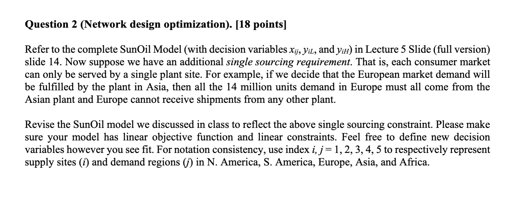
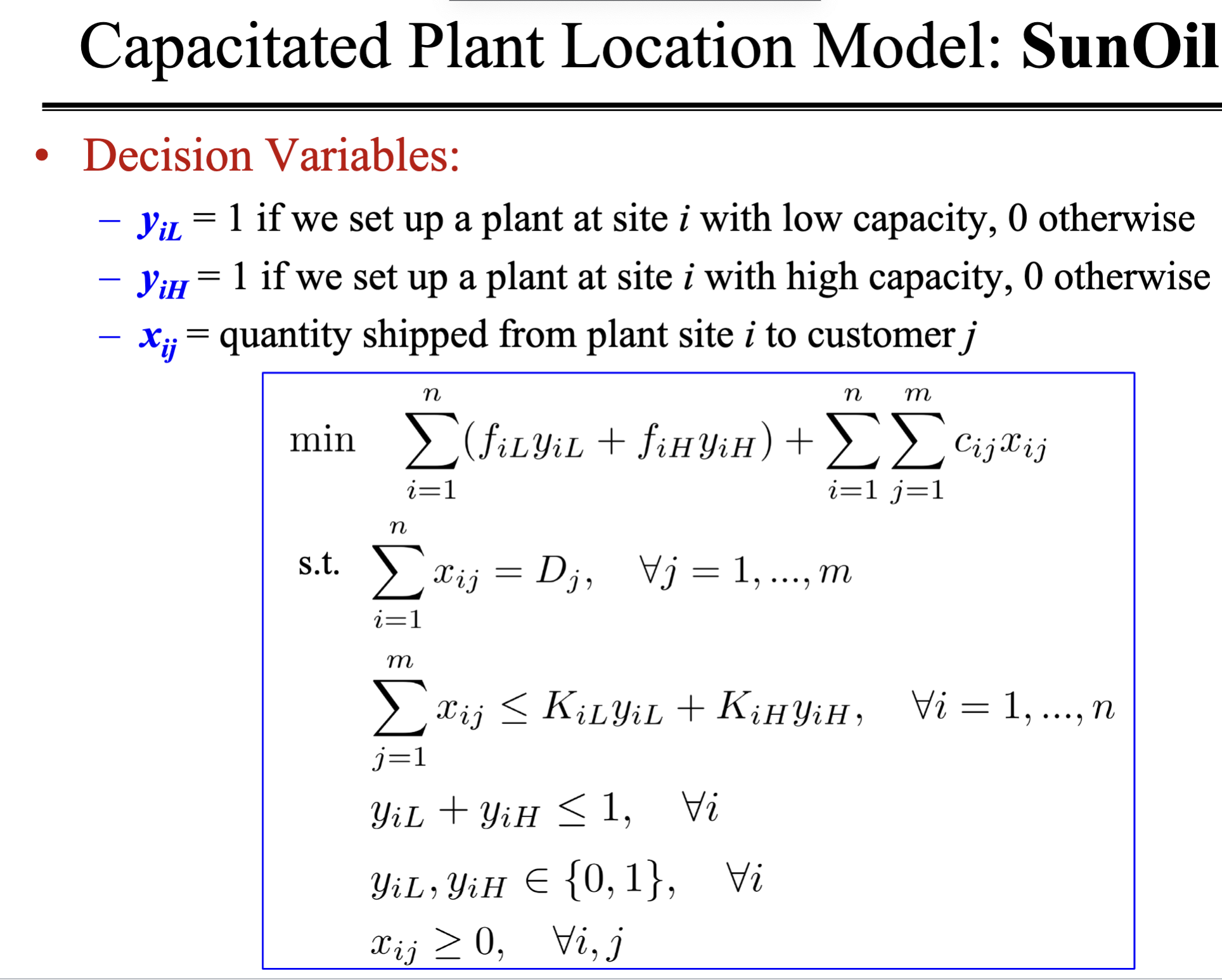
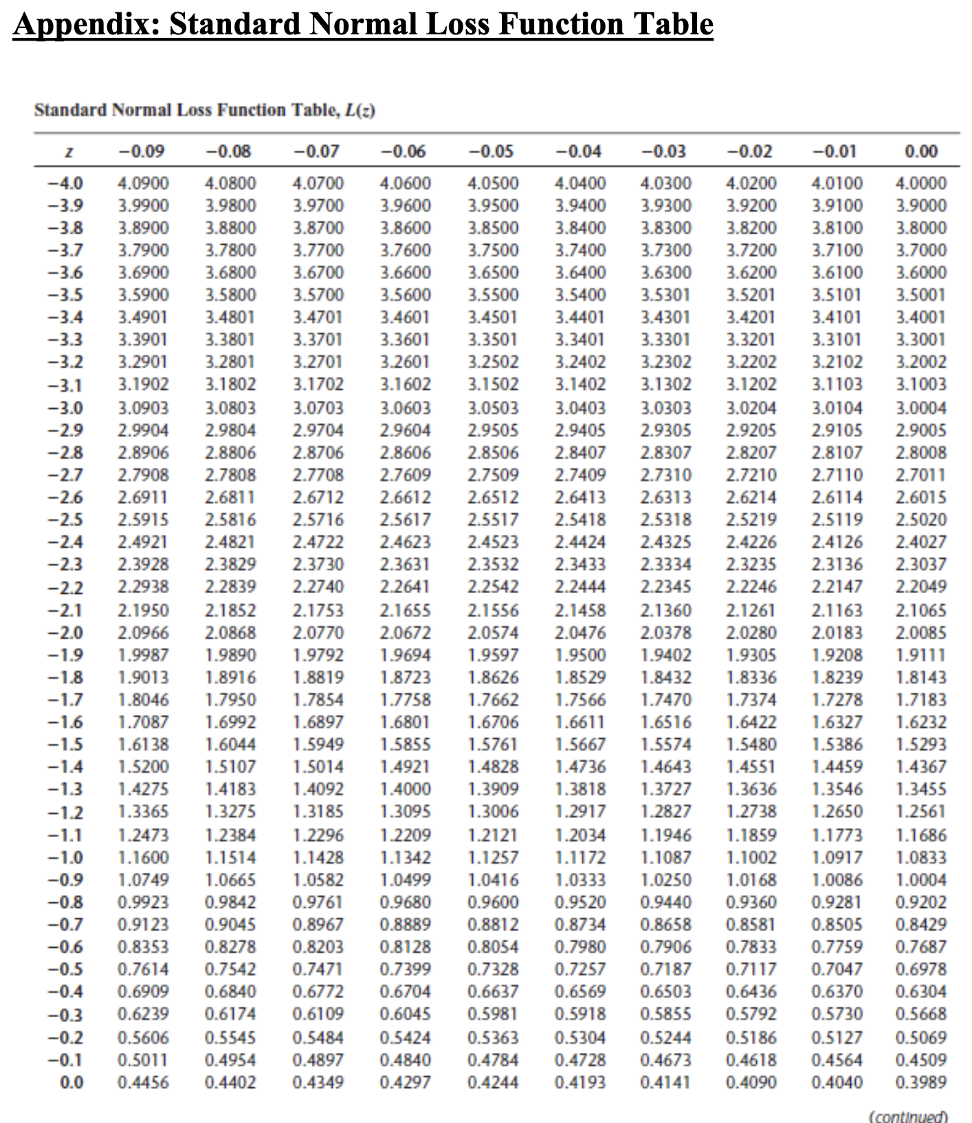
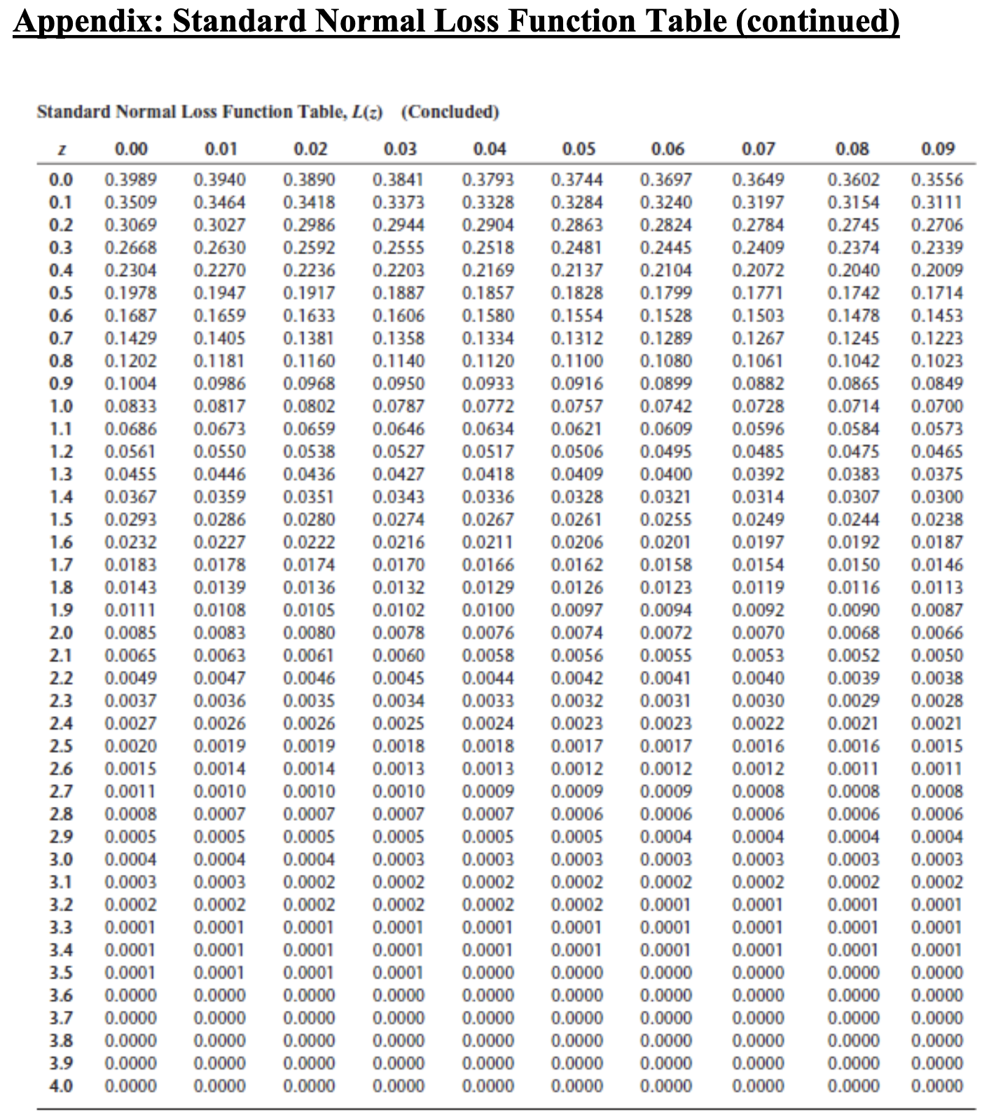
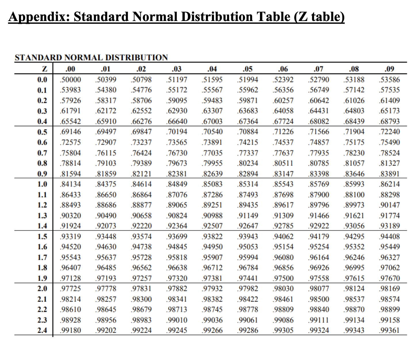
Appendix: Standard Normal Loss Function Table Appendix: Standard Normal Loss Function $Table (continued) Standard Normal Loss Function Table, L(z) (Concluded) \begin{tabular}{|c|c|c|c|c|c|c|c|c|c|c|} \hlinez &$ 0.00 & 0.01 & 0.02 & 0.03 & 0.04 & 0.05 & $0.06 & 0.07 & 0.08 & 0.09 \\ \hline 0.0 & 0.3989$ & 0.3940 & 0.3890 & 0.3841 & 0.3793 & 0.3744 & 0.3697

Appendix: Standard Normal Loss Function Table Appendix: Standard Normal Loss Function Table (continued) Standard Normal Loss Function Table, L(z) (Concluded) \begin{tabular}{|c|c|c|c|c|c|c|c|c|c|c|} \hlinez & 0.00 & 0.01 & 0.02 & 0.03 & 0.04 & 0.05 & 0.06 & 0.07 & 0.08 & 0.09 \\ \hline 0.0 & 0.3989 & 0.3940 & 0.3890 & 0.3841 & 0.3793 & 0.3744 & 0.3697 & 0.3649 & 0.3602 & 0.3556 \\ \hline 0.1 & 0.3509 & 0.3464 & 0.3418 & 0.3373 & 0.3328 & 0.3284 & 0.3240 & 0.3197 & 0.3154 & 0.3111 \\ \hline 0.2 & 0.3069 & 0.3027 & 0.2986 & 0.2944 & 0.2904 & 0.2863 & 0.2824 & 0.2784 & 0.2745 & 0.2706 \\ \hline 0.3 & 0.2668 & 0.2630 & 0.2592 & 0.2555 & 0.2518 & 0.2481 & 0.2445 & 0.2409 & 0.2374 & 0.2339 \\ \hline 0.4 & 0.2304 & 0.2270 & 0.2236 & 0.2203 & 0.2169 & 0.2137 & 0.2104 & 0.2072 & 0.2040 & 0.2009 \\ \hline 0.5 & 0.1978 & 0.1947 & 0.1917 & 0.1887 & 0.1857 & 0.1828 & 0.1799 & 0.1771 & 0.1742 & 0.1714 \\ \hline 0.6 & 0.1687 & 0.1659 & 0.1633 & 0.1606 & 0.1580 & 0.1554 & 0.1528 & 0.1503 & 0.1478 & 0.1453 \\ \hline 0.7 & 0.1429 & 0.1405 & 0.1381 & 0.1358 & 0.1334 & 0.1312 & 0.1289 & 0.1267 & 0.1245 & 0.1223 \\ \hline 0.8 & 0.1202 & 0.1181 & 0.1160 & 0.1140 & 0.1120 & 0.1100 & 0.1080 & 0.1061 & 0.1042 & 0.1023 \\ \hline 0.9 & 0.1004 & 0.0986 & 0.0968 & 0.0950 & 0.0933 & 0.0916 & 0.0899 & 0.0882 & 0.0865 & 0.0849 \\ \hline 1.0 & 0.0833 & 0.0817 & 0.0802 & 0.0787 & 0.0772 & 0.0757 & 0.0742 & 0.0728 & 0.0714 & 0.0700 \\ \hline 1.1 & 0.0686 & 0.0673 & 0.0659 & 0.0646 & 0.0634 & 0.0621 & 0.0609 & 0.0596 & 0.0584 & 0.0573 \\ \hline 1.2 & 0.0561 & 0.0550 & 0.0538 & 0.0527 & 0.0517 & 0.0506 & 0.0495 & 0.0485 & 0.0475 & 0.0465 \\ \hline 1.3 & 0.0455 & 0.0446 & 0.0436 & 0.0427 & 0.0418 & 0.0409 & 0.0400 & 0.0392 & 0.0383 & 0.0375 \\ \hline 1.4 & 0.0367 & 0.0359 & 0.0351 & 0.0343 & 0.0336 & 0.0328 & 0.0321 & 0.0314 & 0.0307 & 0.0300 \\ \hline 1.5 & 0.0293 & 0.0286 & 0.0280 & 0.0274 & 0.0267 & 0.0261 & 0.0255 & 0.0249 & 0.0244 & 0.0238 \\ \hline 1.6 & 0.0232 & 0.0227 & 0.0222 & 0.0216 & 0.0211 & 0.0206 & 0.0201 & 0.0197 & 0.0192 & 0.0187 \\ \hline 1.7 & 0.0183 & 0.0178 & 0.0174 & 0.0170 & 0.0166 & 0.0162 & 0.0158 & 0.0154 & 0.0150 & 0.0146 \\ \hline 1.8 & 0.0143 & 0.0139 & 0.0136 & 0.0132 & 0.0129 & 0.0126 & 0.0123 & 0.0119 & 0.0116 & 0.0113 \\ \hline 1.9 & 0.0111 & 0.0108 & 0.0105 & 0.0102 & 0.0100 & 0.0097 & 0.0094 & 0.0092 & 0.0090 & 0.0087 \\ \hline 2.0 & 0.0085 & 0.0083 & 0.0080 & 0.0078 & 0.0076 & 0.0074 & 0.0072 & 0.0070 & 0.0068 & 0.0066 \\ \hline 2.1 & 0.0065 & 0.0063 & 0.0061 & 0.0060 & 0.0058 & 0.0056 & 0.0055 & 0.0053 & 0.0052 & 0.0050 \\ \hline 2.2 & 0.0049 & 0.0047 & 0.0046 & 0.0045 & 0.0044 & 0.0042 & 0.0041 & 0.0040 & 0.0039 & 0.0038 \\ \hline 2.3 & 0.0037 & 0.0036 & 0.0035 & 0.0034 & 0.0033 & 0.0032 & 0.0031 & 0.0030 & 0.0029 & 0.0028 \\ \hline 2.4 & 0.0027 & 0.0026 & 0.0026 & 0.0025 & 0.0024 & 0.0023 & 0.0023 & 0.0022 & 0.0021 & 0.0021 \\ \hline 2.5 & 0.0020 & 0.0019 & 0.0019 & 0.0018 & 0.0018 & 0.0017 & 0.0017 & 0.0016 & 0.0016 & 0.0015 \\ \hline 2.6 & 0.0015 & 0.0014 & 0.0014 & 0.0013 & 0.0013 & 0.0012 & 0.0012 & 0.0012 & 0.0011 & 0.0011 \\ \hline 2.7 & 0.0011 & 0.0010 & 0.0010 & 0.0010 & 0.0009 & 0.0009 & 0.0009 & 0.0008 & 0.0008 & 0.0008 \\ \hline 2.8 & 0.0008 & 0.0007 & 0.0007 & 0.0007 & 0.0007 & 0.0006 & 0.0006 & 0.0006 & 0.0006 & 0.0006 \\ \hline 2.9 & 0.0005 & 0.0005 & 0.0005 & 0.0005 & 0.0005 & 0.0005 & 0.0004 & 0.0004 & 0.0004 & 0.0004 \\ \hline 3.0 & 0.0004 & 0.0004 & 0.0004 & 0.0003 & 0.0003 & 0.0003 & 0.0003 & 0.0003 & 0.0003 & 0.0003 \\ \hline 3.1 & 0.0003 & 0.0003 & 0.0002 & 0.0002 & 0.0002 & 0.0002 & 0.0002 & 0.0002 & 0.0002 & 0.0002 \\ \hline 3.2 & 0.0002 & 0.0002 & 0.0002 & 0.0002 & 0.0002 & 0.0002 & 0.0001 & 0.0001 & 0.0001 & 0.0001 \\ \hline 3.3 & 0.0001 & 0.0001 & 0.0001 & 0.0001 & 0.0001 & 0.0001 & 0.0001 & 0.0001 & 0.0001 & 0.0001 \\ \hline 3.4 & 0.0001 & 0.0001 & 0.0001 & 0.0001 & 0.0001 & 0.0001 & 0.0001 & 0.0001 & 0.0001 & 0.0001 \\ \hline 3.5 & 0.0001 & 0.0001 & 0.0001 & 0.0001 & 0.0000 & 0.0000 & 0.0000 & 0.0000 & 0.0000 & 0.0000 \\ \hline 3.6 & 0.0000 & 0.0000 & 0.0000 & 0.0000 & 0.0000 & 0.0000 & 0.0000 & 0.0000 & 0.0000 & 0.0000 \\ \hline 3.7 & 0.0000 & 0.0000 & 0.0000 & 0.0000 & 0.0000 & 0.0000 & 0.0000 & 0.0000 & 0.0000 & 0.0000 \\ \hline 3.8 & 0.0000 & 0.0000 & 0.0000 & 0.0000 & 0.0000 & 0.0000 & 0.0000 & 0.0000 & 0.0000 & 0.0000 \\ \hline 3.9 & 0.0000 & 0.0000 & 0.0000 & 0.0000 & 0.0000 & 0.0000 & 0.0000 & 0.0000 & 0.0000 & 0.0000 \\ \hline 4.0 & 0.0000 & 0.0000 & 0.0000 & 0.0000 & 0.0000 & 0.0000 & 0.0000 & 0.0000 & 0.0000 & 0.0000 \\ \hline \end{tabular} Capacitated Plant Location Model: SunOil Decision Variables: yiL=1 if we set up a plant at site i with low capacity, 0 otherwise yiH=1 if we set up a plant at site i with high capacity, 0 otherwise xij= quantity shipped from plant site i to customer j mini=1n(fiLyiL+fiHyiH)+i=1nj=1mcijxijs.t.i=1nxij=Dj,j=1,,mj=1mxijKiLyiL+KiHyiH,i=1,,nyiL+yiH1,iyiL,yiH{0,1},ixij0,i,j Question 2 (Network design optimization). [18 points] Refer to the complete SunOil Model (with decision variables xij,yiL, and yiH ) in Lecture 5 Slide (full version) slide 14. Now suppose we have an additional single sourcing requirement. That is, each consumer market can only be served by a single plant site. For example, if we decide that the European market demand will be fulfilled by the plant in Asia, then all the 14 million units demand in Europe must all come from the Asian plant and Europe cannot receive shipments from any other plant. Revise the SunOil model we discussed in class to reflect the above single sourcing constraint. Please make sure your model has linear objective function and linear constraints. Feel free to define new decision variables however you see fit. For notation consistency, use index i,j=1,2,3,4,5 to respectively represent supply sites (i) and demand regions (j) in N. America, S. America, Europe, Asia, and Africa. Appendix: Standard Normal Distribution Table ( Z table)

Step by Step Solution

There are 3 Steps involved in it

1 Expert Approved Answer

Step: 1 Unlock blur-text-image

Question Has Been Solved by an Expert!

Get step-by-step solutions from verified subject matter experts

Step: 2 Unlock

Step: 3 Unlock

Students Have Also Explored These Related General Management Questions!

Appendix: Standard Normal Loss Function Table (continued) Standard Normal Loss Function Table, L(z) (Concluded) \begin{tabular}{|c|c|c|c|c|c|c|c|c|c|c|} \hlinez & 0.00 & 0.01 & 0.02 & 0.03 & 0.04 &...

Appendix: Standard Normal Loss Function Table Appendix: Standard Normal Distribution Table ( Z table) The All-Colorful Company produces a variety of paint products. Demand is highly seasonal, and the...

Appendix: Standard Normal Loss Function Table Appendix: Standard Normal Distribution Table ( Z table) Question 5 (Risk Pooling Strategies). [8 points] An apparel company is selling a newly designed...

Appendix: Standard Normal Loss Function Table Appendix: Standard Normal Distribution Table ( Z table) Appendix: Standard Normal Loss Function Table (continued) Standard Normal Loss Function Table,...

Question 3 (Inventory Management I). [20 points] Rainbow Colors paint store uses a continuous review inventory system to control its stock levels. For a popular eggshell latex paint, historical data...

Appendix: Standard Normal Loss Function Table (continued) Standard Normal Loss Function Table, L(z) (Concluded) Z 0.00 0.01 0.02 0.03 0.04 0.05 0.06 0.07 0.08 0.09 0.0 0.3989 0.3940 0.3890 0.3841...

Please confirm the answer for question 3 and the rest of the question. I need an expert tutor to look over my solution You are a newsvendor selling the San Pedro Times every morning. Before you get...

*i always give THUMBS UP but please show work (: * news-vendor model This catalog/internet retailer must make a decision on how many -high end, pre-lit fake Christmas trees to buy for the season....

Here are the percentages of Americans who are obese for the Northeastern and Midwestern states: For parts (a), (b) and (c), begin with lower class limit 22 and class width 2. a. Construct a frequency...

A sample consisting of five molecules has a total energy SE. Each molecule is able to occupy states of energy jE, with j = 0, 1,2, .... (a) Calculate the weight of the configuration in which the...

An architect who fails to pay her annual license renewal fee will be unable to collect fees for work done until the renewal fee is paid.

Premise: Using a dictionary and list, create a set of key / value pairs that consists of a musical database. The key / value pairs should consist of Artist Name: Song Names pattern. For example, EACH...