

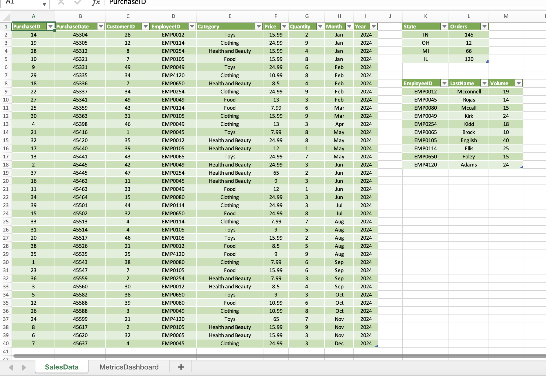
Question: In the Power Pivot window, create a Chart and Table (Horizontal) combination on the MetricsDashboard worksheet in cell B2. In the PivotChart, drag the Category
| In the Power Pivot window, create a Chart and Table (Horizontal) combination on the MetricsDashboard worksheet in cell B2. In the PivotChart, drag the Category field from SalesData2024 to the Axis (Categories) area. Drag the Quantity field from SalesData2024 to the Values area to calculate the sum of quantity sold. Change the chart type to a Pie chart. Apply Style 9 to the PivotChart. Add a Chart Title that reads Volume Sales by Category. Add a Timeline slicer connected to the PivotChart, select the PurchaseDate check box, and position it below the chart. Apply the Light Green, Timeline Style Light 6 to the slicer. | 15 |
| 8 | Name the PivotTable EmployeeRevGoals. Drag the LastName field from VolumeByEmp to the Rows area. Drag the Sum of Revenue Value field from SalesData2024 to the Values area. Drag the Sum of Revenue KPI Status field to the Values area. Rename the Row Labels heading in J2 to Employees. Rename the Sum of Revenue heading in K2 to 2024 Revenue. Rename the Sum of Revenue Status heading in L2 as $500 Goal Status. If necessary, resize the column to fit the text. Apply the PivotTable Style, Light Green, Pivot Style Medium 14 to the PivotTable. |
SalesData MetricsDashboard
Step by Step Solution
There are 3 Steps involved in it
1 Expert Approved Answer
Step: 1 Unlock

Question Has Been Solved by an Expert!
Get step-by-step solutions from verified subject matter experts
Step: 2 Unlock
Step: 3 Unlock