Please explain each step.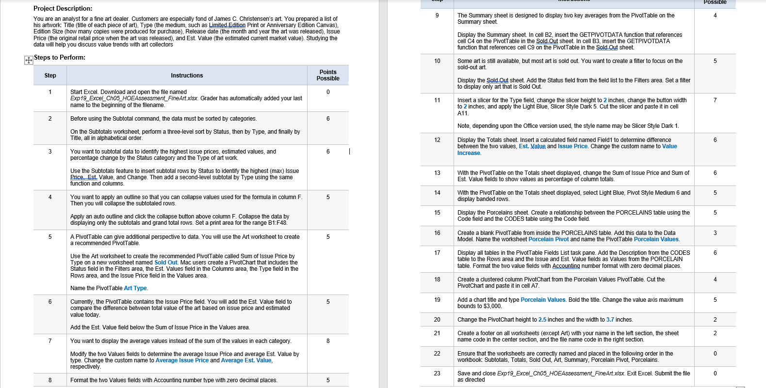

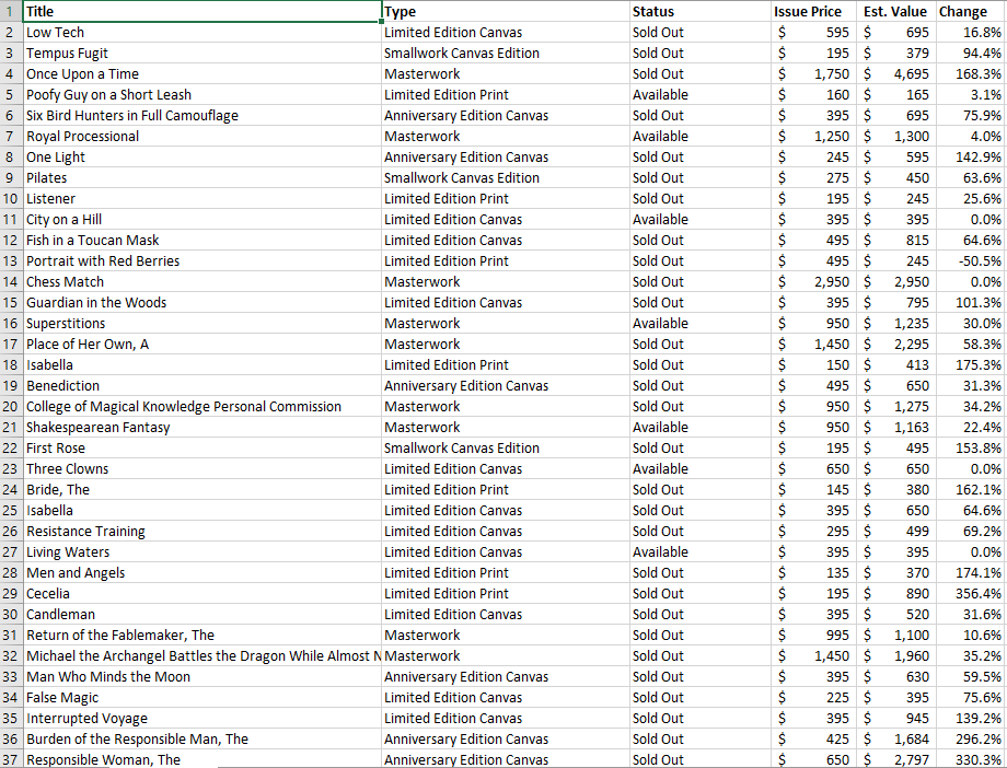
Possible 9 4 The Summary sheet is designed to display two key averages from the PivotTable on the Summary sheet. Project Description: You are an analyst for a fine art dealer. Customers are especially fond of James C. Christensen's art. You prepared a list of his artwork: Title (title of each piece of art), Type (the medium, such as Limited Edition Print or Anniversary Edition Canvas), Edition Size (how many copies were produced for purchase), Release date (the month and year the art was released), Issue Price (the original retail price when the art was released), and Est Value (the estimated current market value). Studying the data will help you discuss value trends with art collectors Steps to Perform: Display the Summary sheet. In cell B2, insert the GETPIVOTDATA function that references cell CA on the PivotTable in the Sold Out sheet. In cell B3, insert the GETPIVOTDATA function that references cell C9 on the Pivot Table in the Sold Out sheet. 10 5 Some art is still available, but most art is sold out. You want to create a filter to focus on the sold-out art Step Instructions Points Possible Display the Sold Out sheet. Add the Status field from the field list to the Filters area. Set a filter to display only art that is Sold Out. 1 0 11 7 Start Excel. Download and open the file named Exp19_Excel_Ch05_HOEAssessment_FineArt.xlsx. Grader has automatically added your last name to the beginning of the filename. Before using the Subtotal command, the data must be sorted by categories. On the Subtotals worksheet, perform a three-level sort by Status, then by Type, and finally by Title, all in alphabetical order. Insert a slicer for the Type field, change the slicer height to 2 inches, change the button width to 2 inches, and apply the Light Blue, Slicer Style Dark 5. Cut the slicer and paste it in cell A11. 2 6 6 Note, depending upon the Office version used, the style name may be Slicer Style Dark 1. 12 6 Display the Totals sheet. Insert a calculated field named Field1 to determine difference between the two values, Est. Value and Issue Price. Change the custom name to Value Increase. 3 6 1 You want to subtotal data to identify the highest issue prices, estimated values, and percentage change by the Status category and the Type of art work. Use the Subtotals feature to insert subtotal rows by Status to identify the highest (max) Issue Price. Est.Value, and Change. Then add a second-level subtotal by Type using the same function and columns 13 6 With the PivotTable on the Totals sheet displayed, change the Sum of Issue Price and Sum of Est. Value fields to show values as percentage of column totals. 14 5 4 5 With the PivotTable on the Totals sheet displayed, select Light Blue, Pivot Style Medium 6 and display banded rows. You want to apply an outline so that you can collapse values used for the formula in column F. Then you will collapse the subtotaled rows. Apply an auto outline and click the collapse button above column F. Collapse the data by displaying only the subtotals and grand total rows. Set a print area for the range B1:F48. 15 5 Display the Porcelains sheet. Create a relationship between the PORCELAINS table using the Code field and the CODES table using the Code field. 16 3 5 5 A PivotTable can give additional perspective to data. You will use the Art worksheet to create a recommended PivotTable. 17 Create a blank PivotTable from inside the PORCELAINS table. Add this data to the Data Model. Name the worksheet Porcelain Pivot and name the PivotTable Porcelain Values. Display all tables in the PivotTable Fields List task pane. Add the Description from the CODES table to the Rows area and the issue and Est Value fields as Values from the PORCELAIN table. Format the two value fields with Accounting number format with zero decimal places. 6 Use the Art worksheet to create the recommended PivotTable called Sum of Issue Price by Type on a new worksheet named Sold Out. Mac users create a PivotChart that includes the Status field in the Filters area, the Est. Values field in the Columns area, the Type field in the Rows area, and the issue Price field in the Values area. 18 4 Create a clustered column PivotChart from the Porcelain Values PivotTable. Cut the PivotChart and paste it in cell A7 6 Name the PivotTable Art Type. Currently, the PivotTable contains the issue Price field. You will add the Est Value field to compare the difference between total value of the art based on issue price and estimated value today 5 19 5 Add a chart title and type Porcelain Values. Bold the title. Change the value axis maximum bounds to $3,000. 20 Change the PivotChart height to 2.5 inches and the width to 3.7 inches. 2 Add the Est. Value field below the Sum of Issue Price in the Values area. 21 2 Create a footer on all worksheets (except Art) with your name in the left section, the sheet name code in the center section, and the file name code in the right section. 7 8 You want to display the average values instead of the sum of the values in each category. Modify the two Values fields to determine the average Issue Price and average Est. Value by type. Change the custom name to Average Issue Price and Average Est. Value, respectively 22 0 Ensure that the worksheets are correctly named and placed in the following order in the workbook Subtotals, Totals, Sold Out, Art, Summary, Porcelain Pivot, Porcelains. 23 0 Save and close Exp19_Excel_Ch05_HOEAssessment_FineArt.xlsx. Exit Excel. Submit the file as directed 8 Format the two Values fields with Accounting number type with zero decimal places 5 1 Title Type 2 Low Tech Limited Edition Canvas 3 Tempus Fugit Smallwork Canvas Edition 4 Once Upon a Time Masterwork 5 Poofy Guy on a Short Leash Limited Edition Print 6 Six Bird Hunters in Full Camouflage Anniversary Edition Canvas 7 Royal Processional Masterwork 8 One Light Anniversary Edition Canvas 9 Pilates Smallwork Canvas Edition 10 Listener Limited Edition Print 11 City on a Hill Limited Edition Canvas 12 Fish in a Toucan Mask Limited Edition Canvas 13 Portrait with Red Berries Limited Edition Print 14 Chess Match Masterwork 15 Guardian in the Woods Limited Edition Canvas 16 Superstitions Masterwork 17 Place of Her Own, A Masterwork 18 Isabella Limited Edition Print 19 Benediction Anniversary Edition Canvas 20 College of Magical Knowledge Personal Commission Masterwork 21 Shakespearean Fantasy Masterwork 22 First Rose Smallwork Canvas Edition 23 Three Clowns Limited Edition Canvas 24 Bride, The Limited Edition Print 25 Isabella Limited Edition Canvas 26 Resistance Training Limited Edition Canvas 27 Living Waters Limited Edition Canvas 28 Men and Angels Limited Edition Print 29 Cecelia Limited Edition Print 30 Candleman Limited Edition Canvas 31 Return of the Fablemaker, The Masterwork 32 Michael the Archangel Battles the Dragon While Almost N Masterwork 33 Man Who Minds the Moon Anniversary Edition Canvas 34 False Magic Limited Edition Canvas 35 Interrupted Voyage Limited Edition Canvas 36 Burden of the Responsible Man, The Anniversary Edition Canvas 37 Responsible Woman, The Anniversary Edition Canvas Status Sold Out Sold Out Sold Out Available Sold Out Available Sold Out Sold Out Sold Out Available Sold Out Sold Out Sold Out Sold Out Available Sold Out Sold Out Sold Out Sold Out Available Sold Out Available Sold Out Sold Out Sold Out Available Sold Out Sold Out Sold Out Sold Out Sold Out Sold Out Sold Out Sold Out Sold Out Sold Out Issue Price Est. Value Change $ 595 $ 695 16.8% $ 195 $ 379 94.4% $ 1,750 $ 4,695 168.3% $ 160 $ 165 3.1% $ 395 $ 695 75.9% $ 1,250 $ 1,300 4.0% $ 245 $ 595 142.9% $ 275 $ 450 63.6% $ 195 $ 245 25.6% $ 395 $ 395 0.0% $ 495 $ 815 64.6% $ 495 $ 245 -50.5% $ 2,950 $ 2,950 0.0% $ 395 $ 795 101.3% $ 950 $ 1,235 30.0% $ 1,450 $ 2,295 58.3% $ 150 $ 413 175.3% $ 495 $ 650 31.3% $ 950 $ 1,275 34.2% $ 950 $ 1,163 22.4% $ 195 $ 495 153.8% $ 650 $ 650 0.0% $ 145 $ 380 162.1% $ 395 $ 650 64.6% $ 295 $ 499 69.2% $ 395 $ 395 0.0% $ 135 S 370 174.1% $ 195 $ 890 356.4% $ 395 $ 520 31.6% $ 995 $ 1,100 10.6% $ 1,450 $ 1,960 35.2% $ 395 $ 630 59.5% $ 225 $ 395 75.6% $ 395 $ 945 139.2% $ 425 $ 1,684 296.2% $ 650 $ 2,797 330.3% Possible 9 4 The Summary sheet is designed to display two key averages from the PivotTable on the Summary sheet. Project Description: You are an analyst for a fine art dealer. Customers are especially fond of James C. Christensen's art. You prepared a list of his artwork: Title (title of each piece of art), Type (the medium, such as Limited Edition Print or Anniversary Edition Canvas), Edition Size (how many copies were produced for purchase), Release date (the month and year the art was released), Issue Price (the original retail price when the art was released), and Est Value (the estimated current market value). Studying the data will help you discuss value trends with art collectors Steps to Perform: Display the Summary sheet. In cell B2, insert the GETPIVOTDATA function that references cell CA on the PivotTable in the Sold Out sheet. In cell B3, insert the GETPIVOTDATA function that references cell C9 on the Pivot Table in the Sold Out sheet. 10 5 Some art is still available, but most art is sold out. You want to create a filter to focus on the sold-out art Step Instructions Points Possible Display the Sold Out sheet. Add the Status field from the field list to the Filters area. Set a filter to display only art that is Sold Out. 1 0 11 7 Start Excel. Download and open the file named Exp19_Excel_Ch05_HOEAssessment_FineArt.xlsx. Grader has automatically added your last name to the beginning of the filename. Before using the Subtotal command, the data must be sorted by categories. On the Subtotals worksheet, perform a three-level sort by Status, then by Type, and finally by Title, all in alphabetical order. Insert a slicer for the Type field, change the slicer height to 2 inches, change the button width to 2 inches, and apply the Light Blue, Slicer Style Dark 5. Cut the slicer and paste it in cell A11. 2 6 6 Note, depending upon the Office version used, the style name may be Slicer Style Dark 1. 12 6 Display the Totals sheet. Insert a calculated field named Field1 to determine difference between the two values, Est. Value and Issue Price. Change the custom name to Value Increase. 3 6 1 You want to subtotal data to identify the highest issue prices, estimated values, and percentage change by the Status category and the Type of art work. Use the Subtotals feature to insert subtotal rows by Status to identify the highest (max) Issue Price. Est.Value, and Change. Then add a second-level subtotal by Type using the same function and columns 13 6 With the PivotTable on the Totals sheet displayed, change the Sum of Issue Price and Sum of Est. Value fields to show values as percentage of column totals. 14 5 4 5 With the PivotTable on the Totals sheet displayed, select Light Blue, Pivot Style Medium 6 and display banded rows. You want to apply an outline so that you can collapse values used for the formula in column F. Then you will collapse the subtotaled rows. Apply an auto outline and click the collapse button above column F. Collapse the data by displaying only the subtotals and grand total rows. Set a print area for the range B1:F48. 15 5 Display the Porcelains sheet. Create a relationship between the PORCELAINS table using the Code field and the CODES table using the Code field. 16 3 5 5 A PivotTable can give additional perspective to data. You will use the Art worksheet to create a recommended PivotTable. 17 Create a blank PivotTable from inside the PORCELAINS table. Add this data to the Data Model. Name the worksheet Porcelain Pivot and name the PivotTable Porcelain Values. Display all tables in the PivotTable Fields List task pane. Add the Description from the CODES table to the Rows area and the issue and Est Value fields as Values from the PORCELAIN table. Format the two value fields with Accounting number format with zero decimal places. 6 Use the Art worksheet to create the recommended PivotTable called Sum of Issue Price by Type on a new worksheet named Sold Out. Mac users create a PivotChart that includes the Status field in the Filters area, the Est. Values field in the Columns area, the Type field in the Rows area, and the issue Price field in the Values area. 18 4 Create a clustered column PivotChart from the Porcelain Values PivotTable. Cut the PivotChart and paste it in cell A7 6 Name the PivotTable Art Type. Currently, the PivotTable contains the issue Price field. You will add the Est Value field to compare the difference between total value of the art based on issue price and estimated value today 5 19 5 Add a chart title and type Porcelain Values. Bold the title. Change the value axis maximum bounds to $3,000. 20 Change the PivotChart height to 2.5 inches and the width to 3.7 inches. 2 Add the Est. Value field below the Sum of Issue Price in the Values area. 21 2 Create a footer on all worksheets (except Art) with your name in the left section, the sheet name code in the center section, and the file name code in the right section. 7 8 You want to display the average values instead of the sum of the values in each category. Modify the two Values fields to determine the average Issue Price and average Est. Value by type. Change the custom name to Average Issue Price and Average Est. Value, respectively 22 0 Ensure that the worksheets are correctly named and placed in the following order in the workbook Subtotals, Totals, Sold Out, Art, Summary, Porcelain Pivot, Porcelains. 23 0 Save and close Exp19_Excel_Ch05_HOEAssessment_FineArt.xlsx. Exit Excel. Submit the file as directed 8 Format the two Values fields with Accounting number type with zero decimal places 5 1 Title Type 2 Low Tech Limited Edition Canvas 3 Tempus Fugit Smallwork Canvas Edition 4 Once Upon a Time Masterwork 5 Poofy Guy on a Short Leash Limited Edition Print 6 Six Bird Hunters in Full Camouflage Anniversary Edition Canvas 7 Royal Processional Masterwork 8 One Light Anniversary Edition Canvas 9 Pilates Smallwork Canvas Edition 10 Listener Limited Edition Print 11 City on a Hill Limited Edition Canvas 12 Fish in a Toucan Mask Limited Edition Canvas 13 Portrait with Red Berries Limited Edition Print 14 Chess Match Masterwork 15 Guardian in the Woods Limited Edition Canvas 16 Superstitions Masterwork 17 Place of Her Own, A Masterwork 18 Isabella Limited Edition Print 19 Benediction Anniversary Edition Canvas 20 College of Magical Knowledge Personal Commission Masterwork 21 Shakespearean Fantasy Masterwork 22 First Rose Smallwork Canvas Edition 23 Three Clowns Limited Edition Canvas 24 Bride, The Limited Edition Print 25 Isabella Limited Edition Canvas 26 Resistance Training Limited Edition Canvas 27 Living Waters Limited Edition Canvas 28 Men and Angels Limited Edition Print 29 Cecelia Limited Edition Print 30 Candleman Limited Edition Canvas 31 Return of the Fablemaker, The Masterwork 32 Michael the Archangel Battles the Dragon While Almost N Masterwork 33 Man Who Minds the Moon Anniversary Edition Canvas 34 False Magic Limited Edition Canvas 35 Interrupted Voyage Limited Edition Canvas 36 Burden of the Responsible Man, The Anniversary Edition Canvas 37 Responsible Woman, The Anniversary Edition Canvas Status Sold Out Sold Out Sold Out Available Sold Out Available Sold Out Sold Out Sold Out Available Sold Out Sold Out Sold Out Sold Out Available Sold Out Sold Out Sold Out Sold Out Available Sold Out Available Sold Out Sold Out Sold Out Available Sold Out Sold Out Sold Out Sold Out Sold Out Sold Out Sold Out Sold Out Sold Out Sold Out Issue Price Est. Value Change $ 595 $ 695 16.8% $ 195 $ 379 94.4% $ 1,750 $ 4,695 168.3% $ 160 $ 165 3.1% $ 395 $ 695 75.9% $ 1,250 $ 1,300 4.0% $ 245 $ 595 142.9% $ 275 $ 450 63.6% $ 195 $ 245 25.6% $ 395 $ 395 0.0% $ 495 $ 815 64.6% $ 495 $ 245 -50.5% $ 2,950 $ 2,950 0.0% $ 395 $ 795 101.3% $ 950 $ 1,235 30.0% $ 1,450 $ 2,295 58.3% $ 150 $ 413 175.3% $ 495 $ 650 31.3% $ 950 $ 1,275 34.2% $ 950 $ 1,163 22.4% $ 195 $ 495 153.8% $ 650 $ 650 0.0% $ 145 $ 380 162.1% $ 395 $ 650 64.6% $ 295 $ 499 69.2% $ 395 $ 395 0.0% $ 135 S 370 174.1% $ 195 $ 890 356.4% $ 395 $ 520 31.6% $ 995 $ 1,100 10.6% $ 1,450 $ 1,960 35.2% $ 395 $ 630 59.5% $ 225 $ 395 75.6% $ 395 $ 945 139.2% $ 425 $ 1,684 296.2% $ 650 $ 2,797 330.3%