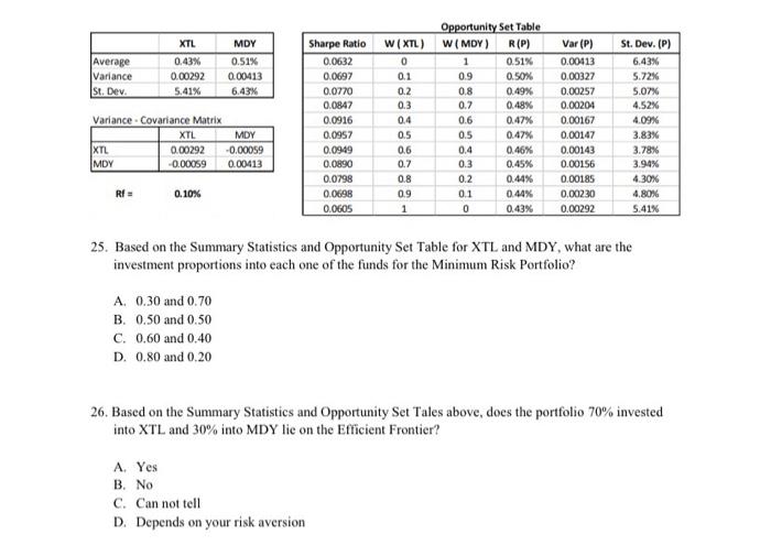
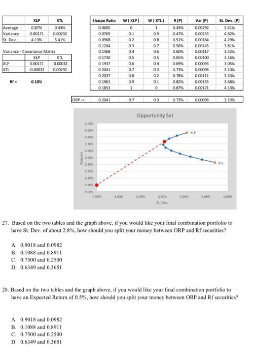
XTL Average Variance St. Dev. 0.43% 0.00292 5.41% MDY 0.51% 0.00413 6.43% Variance - Covariance Matrix XTL MDY 0.00292 -0.00059 -0.00059 0.00413 Sharpe Ratio 0.0632 0.0697 0.0770 0.0847 0.0916 0.0957 0.0949 0.0890 0.0798 0.0698 0 OGOS W(XTL) 0 0.1 0.2 0.3 0.4 0.5 0.6 0.7 0.8 0.9 1 Opportunity Set Table W(MDY) R(P) 0.51% 09 0.50% 0.8 0.49% 0.7 0.48% 0.6 0.47% 0.5 0.47% 0.4 0.46% 0.3 0.45% 0.2 0.44% 0.1 0.44% 0 0.43% Var (P) 0.00413 0.00327 0.00257 0.00204 0.00167 0.00147 0.00143 0.00156 0.00185 0.00230 0.00292 St. Dev. (P) 6.43% 5.72% 5.07% 4.52% 4.09% 3.83% 3.78% 3.94% 4.30% 4,80% 5.41% XTL MDY w Rf 0.10% 09 25. Based on the Summary Statistics and Opportunity Set Table for XTL and MDY, what are the investment proportions into each one of the funds for the Minimum Risk Portfolio? A. 0.30 and 0.70 B. 0.50 and 0.50 C. 0.60 and 0.40 D. 0.80 and 0.20 26. Based on the Summary Statistics and Opportunity Set Tales above, does the portfolio 70% invested into XTL and 30% into MDY lie on the Efficient Frontier? A. Yes B. No C. Can not tell D. Depends on your risk aversion Average Variance St. Dev. XLP 0.87% 0.00171 4.13% XTL 0.43% 0.00292 5.4156 Variance - Covariance Matrix XLP XTL 0.00171 0.00032 -0.00032 0.00292 Sharpe Ratio 0.0605 0.0769 0.0958 0.1204 0.1468 0.1730 0.1937 0.2041 0.2037 0.1961 0.1853 W(XLP) 0 0.1 0.2 03 0.4 OS 0.6 0.2 0.8 09 1 W(TL) 1 0.9 0.8 0.7 0.6 05 0.4 0.3 02 0.1 0 RIP) 0.43% 0.47% 0.51% 0.56% 0.60% 0.65% 0.69% 0.73% 0.78% 0.82% 0.87% Var (P) 0.00292 0.00233 0.00184 0.00145 0.00117 0.00100 0.00093 0.00096 0.00111 0.00135 0.00171 St. Dev. (P) 5.41% 4.82% 4.29% 3.81% 3.42% 3.16% 3.05% 3.10% 3.33% 3.68 413 XLP XTL RI 0.10% B ORP 0.2011 0.7 0.73% 0.00096 3.10% Opportunity Set 1.00 XLP GRON OTON . BON XTL 20N .LON O.COM DON 1.00 2.00 300 4.00 500 OON $t. Dey 27. Based on the two tables and the graph above, if you would like your final combination portfolio to have St. Dev. of about 2.8%, how should you split your money between ORP and Rf securities? A. 0.9018 and 0.0982 B. 0.1088 and 0.8911 C. 0.7500 and 0.2500 D. 0.6349 and 0.3651 28. Based on the two tables and the graph above, if you would like your final combination portfolio to have an Expected Return of 0.5%, how should you split your money between ORP and Rf securities? A 0.9018 and 0.0982 B. 0.1088 and 0.8911 C. 0.7500 and 0.2500 D. 0.6349 and 0.3651 29. Based on the two tables and the graph above, what would be the Sharpe Ratio of the 20/80 Final Combination of Rf security and ORP? A. 0.3218 B. 0.2041 C. 0.1599 D. 0.0720 XTL Average Variance St. Dev. 0.43% 0.00292 5.41% MDY 0.51% 0.00413 6.43% Variance - Covariance Matrix XTL MDY 0.00292 -0.00059 -0.00059 0.00413 Sharpe Ratio 0.0632 0.0697 0.0770 0.0847 0.0916 0.0957 0.0949 0.0890 0.0798 0.0698 0 OGOS W(XTL) 0 0.1 0.2 0.3 0.4 0.5 0.6 0.7 0.8 0.9 1 Opportunity Set Table W(MDY) R(P) 0.51% 09 0.50% 0.8 0.49% 0.7 0.48% 0.6 0.47% 0.5 0.47% 0.4 0.46% 0.3 0.45% 0.2 0.44% 0.1 0.44% 0 0.43% Var (P) 0.00413 0.00327 0.00257 0.00204 0.00167 0.00147 0.00143 0.00156 0.00185 0.00230 0.00292 St. Dev. (P) 6.43% 5.72% 5.07% 4.52% 4.09% 3.83% 3.78% 3.94% 4.30% 4,80% 5.41% XTL MDY w Rf 0.10% 09 25. Based on the Summary Statistics and Opportunity Set Table for XTL and MDY, what are the investment proportions into each one of the funds for the Minimum Risk Portfolio? A. 0.30 and 0.70 B. 0.50 and 0.50 C. 0.60 and 0.40 D. 0.80 and 0.20 26. Based on the Summary Statistics and Opportunity Set Tales above, does the portfolio 70% invested into XTL and 30% into MDY lie on the Efficient Frontier? A. Yes B. No C. Can not tell D. Depends on your risk aversion Average Variance St. Dev. XLP 0.87% 0.00171 4.13% XTL 0.43% 0.00292 5.4156 Variance - Covariance Matrix XLP XTL 0.00171 0.00032 -0.00032 0.00292 Sharpe Ratio 0.0605 0.0769 0.0958 0.1204 0.1468 0.1730 0.1937 0.2041 0.2037 0.1961 0.1853 W(XLP) 0 0.1 0.2 03 0.4 OS 0.6 0.2 0.8 09 1 W(TL) 1 0.9 0.8 0.7 0.6 05 0.4 0.3 02 0.1 0 RIP) 0.43% 0.47% 0.51% 0.56% 0.60% 0.65% 0.69% 0.73% 0.78% 0.82% 0.87% Var (P) 0.00292 0.00233 0.00184 0.00145 0.00117 0.00100 0.00093 0.00096 0.00111 0.00135 0.00171 St. Dev. (P) 5.41% 4.82% 4.29% 3.81% 3.42% 3.16% 3.05% 3.10% 3.33% 3.68 413 XLP XTL RI 0.10% B ORP 0.2011 0.7 0.73% 0.00096 3.10% Opportunity Set 1.00 XLP GRON OTON . BON XTL 20N .LON O.COM DON 1.00 2.00 300 4.00 500 OON $t. Dey 27. Based on the two tables and the graph above, if you would like your final combination portfolio to have St. Dev. of about 2.8%, how should you split your money between ORP and Rf securities? A. 0.9018 and 0.0982 B. 0.1088 and 0.8911 C. 0.7500 and 0.2500 D. 0.6349 and 0.3651 28. Based on the two tables and the graph above, if you would like your final combination portfolio to have an Expected Return of 0.5%, how should you split your money between ORP and Rf securities? A 0.9018 and 0.0982 B. 0.1088 and 0.8911 C. 0.7500 and 0.2500 D. 0.6349 and 0.3651 29. Based on the two tables and the graph above, what would be the Sharpe Ratio of the 20/80 Final Combination of Rf security and ORP? A. 0.3218 B. 0.2041 C. 0.1599 D. 0.0720