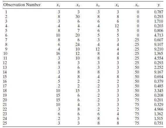
Consider the electronic inverter data in Table B.14. Delete observation 2 from the original data. Electrical engineering theory suggests that we should define new variables as follows: \(y^{*}=\ln y, x_{1}^{*}=1 / \sqrt{x_{1}}, x_{2}^{*}=\sqrt{x_{2}}, x_{3}^{*}=1 / \sqrt{x_{3}}\), and \(x_{4}^{*}=\sqrt{x_{4}}\).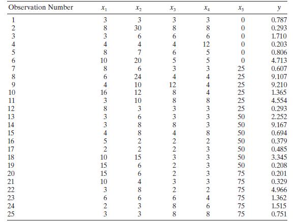

a. Find an appropriate subset regression model for these data using all possible regressions and the \(C_{p}\) criterion.
b. Plot the residuals versus \(\hat{y}^{*}\) for this model. Comment on the plots.
c. Discuss how you could compare this model to the ones built using the original response and regressors in Problem 10.27.

Data From Problem 10.27

Reconsider the electronic inverter data in Table B.14. In Problems 10.24 and 10.25 , you built regression models for the data using different variable selection algorithms. Suppose that you now learn that the second observation was incorrectly recorded and should be ignored.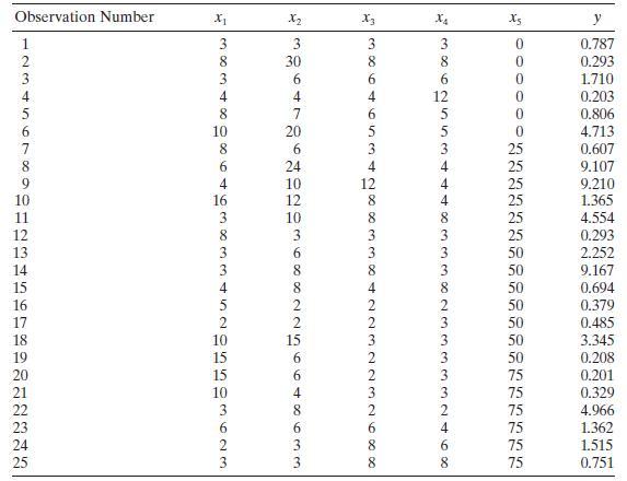

a. Fit a model to the modified data using all possible regressions, using Cp${\mathrm{????}}_{\mathrm{????}}$ as the criterion. Compare this model to the model you found in Problem 10.24.
b. Use stepwise regression to find an appropriate model for the modified data. Compare this model to the one you found in Problem 10.25.
c. Calculate the confidence intervals as the mean response for all points in the modified data set. Compare these results with the confidence intervals from Problem 10.26. Discuss your findings.

Problem 10.24

Table B. 14 presents data on the transient points of an electronic inverter. Use all possible regressions and the CpCp????????${\mathrm{????}}_{\mathrm{????}}$ criterion to find an appropriate regression model for these data. Investigate model adequacy using residual plots.

Problem 10.25

Reconsider the electronic inverter data in Table B.14. Use stepwise regression to find an appropriate regression model for these data. Investigate model adequacy using residual plots. Compare this model with the one found by the all-possible-regressions approach in Problem 10.24.

Problem 10.24

Table B. 14 presents data on the transient points of an electronic inverter. Use all possible regressions and the Cp????????${\mathrm{????}}_{\mathrm{????}}$ criterion to find an appropriate regression model for these data. Investigate model adequacy using residual plots.

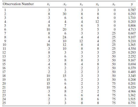
Observation Number x1 X2 X3 xX4 Xs y 1234567890123 3834 386 38 0 0.787 4 8 6 86255 0 0.293 0 1.710 1.710 0 0.203 0 0.600 0.806 123 53428833842232232688 6882256 9864638BLENDER3 0 4.713 0.607 9.107 9.107 9.210 9.210 1.365 4.554 0.293 2.252 9.167 0.694 0.094 0.379 009AN 0.485 3.345 0.208 0.201 33333 0.329 4.966 1.362 1.515 0.751