New Semester
Started
Get
50% OFF
Study Help!
--h --m --s
Claim Now
Question Answers
Textbooks
Find textbooks, questions and answers
Oops, something went wrong!
Change your search query and then try again
S
Books
FREE
Study Help
Expert Questions
Accounting
General Management
Mathematics
Finance
Organizational Behaviour
Law
Physics
Operating System
Management Leadership
Sociology
Programming
Marketing
Database
Computer Network
Economics
Textbooks Solutions
Accounting
Managerial Accounting
Management Leadership
Cost Accounting
Statistics
Business Law
Corporate Finance
Finance
Economics
Auditing
Tutors
Online Tutors
Find a Tutor
Hire a Tutor
Become a Tutor
AI Tutor
AI Study Planner
NEW
Sell Books
Search
Search
Sign In
Register
study help
sciences
solid state physics essential concepts
Solid State Physics Essential Concepts 2nd Edition David W. Snoke - Solutions
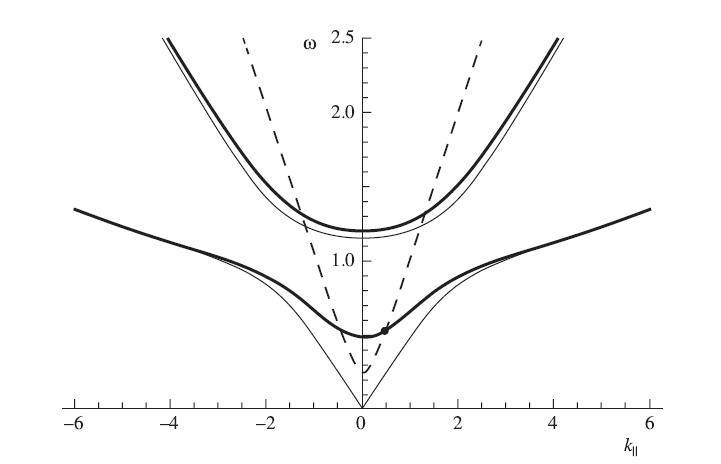
Determine the maximum internal angle of incidence at which a lower polariton can couple to an external photon, as a function of frequency, for the parameters of an exciton-polariton given in Figure 7.15, using a numerical plotting package such as Mathematica. -6 --4 -2 - 2.5 2.0 1.0 0 2 I 4 kj| 6
The complex Fresnel equations allow a powerful method of materials analysis known as ellipsometry. In general, linearly polarized light reflected at an oblique angle will become elliptically polarized, with linear and circular polarization components that depend on the real and imaginary parts of
What acousto-optic figure of merit is needed to get 50% of an input light beam to be redirected into a diffracted beam, if the acoustic intensity is 5 W/cm2? Use the following parameters: The input light has wavelength 600 nm, the index of refraction of the medium is 1.8, the acousto-optic cell
Plot the solutions of (7.5.37) and (7.5.48) as functions of ωk for the same values of Ω = 0.1 and ω0 = 1, and show that they have the same behavior near the crossing of the photon and exciton branches, but differ far from this crossover point. wowk - w(wk + wp) + w ² = = |2₁|²wo/wk =
As discussed above, in time-dependent perturbation theory one can simply drop terms from the lower bounds of all time integrals except the final one, and add a small imaginary term in the denominator consistent with causality. Show that following this procedure for the real part of the third order
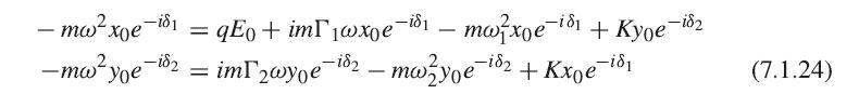
Use a program like Mathematica to solve (7.1.24) for x0, y0, cos δ1, sin δ1, cos δ2, and sin δ2 (subject to the constraints cos2 δ+sin2 δ = 1) and plot the response for qE0 = 1, m = 1, your own choice of parameters ω1,ω2 and the damping constants. -mw² xoe- -i81 -mw²yoe - =
As discussed in Exercise 7.1.2, we can model a metal as an ensemble of classical oscillators with ω0 = 0. Calculate the absolute reflectivity r for an infrared electromagnetic wave, with wavelength 10 μm, incident normal to the surface of a metal with electron density n = 1021 cm−3, electron
How large an effect should acoustic phonons produce? Estimate the polaron mass of electrons at zero temperature due to acoustic phonons, if the band effective mass is equal to the free electron mass, the electron–phonon deformation potential energy is D = 1 eV, the speed of sound is v = 5 × 10⁵
The resonant Raman scattering diagram shown in Figure 8.7(a) can be compared to the results of Section 7.8 by taking the initial state |i〉 as Ni photons in state qvector) and the final state as Ni − 1 photons in state q(vector) and a phonon in state p(vector).(a) Calculate the rate of
Estimate the band shift with temperature due to electron–phonon Fröhlich interaction, for an electron band with effective mass equal to the free electron mass, optical phonon energy h̄ωLO = 30 meV, and ϵ(0)/ϵ0 = 10 and ϵ(∞)/ϵ0 = 1. What is the magnitude of the band shift due to the
What does the transition spectrum look like on short time scales? Instead of taking the limit t → ∞, determine the probability |〈f ψ(t)〉|2, and use a program like Mathematica to plot it as a function of final state energy Ef, for various times t. You should see that at early times the
Verify Wick’s theorem explicitly for two fermion operators acting on the same state k(vector). Show also that bk(t1)b}{(12) = — b}(t2)bk(tr). (8.6.17)
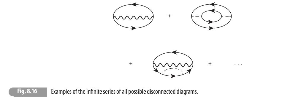
Write down the integral for the second diagram in Figure 8.16 and show that it is nonzero. Fig. 8.16 Examples of the infinite series of all possible disconnected diagrams. +
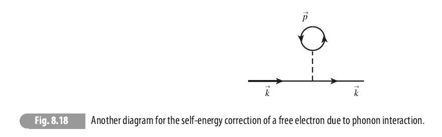
Using the finite-temperature Green’s functions given in this section, compute the real self-energy correction for a free electron that corresponds to the diagram shown in Figure 8.18, known as a “tadpole” diagram, for optical phonons with constant energy h̄ωLO. To have a sensible answer,
Show that (8.11.8) and (8.11.13) both follow from (8.11.12) for an electron gas with two degenerate spin states, in the two limits of a T = 0 electron gas with a Fermi level, and in the high-temperature, Maxwell–Boltzmann limit. 2 K = Зе²п 2EEF (8.11.8)
(a) Verify that (8.12.3) follows from (8.12.2) for the case of a threedimensional electron gas with a Fermi level EF.(b) Use a program like Mathematica to calculate numerically the unscreened exchange energy from (8.12.2) for the case of a Maxwell–Boltzmann distribution of electrons, that is, the
Verify the revised Wick’s theorem (8.13.7) explicitly for the thermal average of four operators, (a (t₁)b (t)b (1₂)a (1₂2)). k
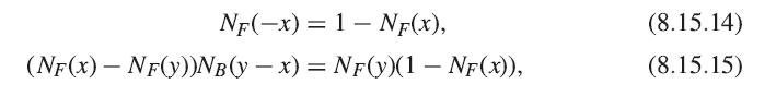
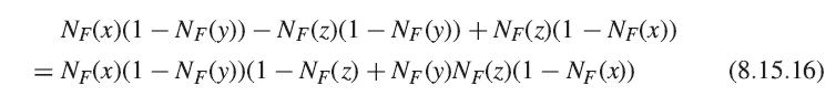
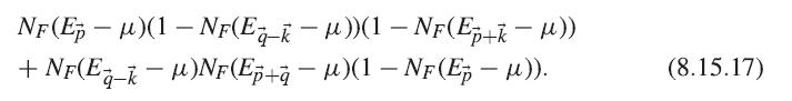
Prove the identities (8.15.14), (8.15.15), and (8.15.16), and therefore the conversion of the occupation number factor in (8.15.13) to (8.15.17). Σ₁ = ΣM² (NF (E₂ − µ) — NƑ(Eñ+k − µ)) p,k X NF (-E-k+μ) + NB (Ep+k - Ep) Ep+k+Ea-k-E₁-E₂- in (8.15.13)
Deduce the existence of the second-order susceptibility χ(2) in (7.6.1), which gives a response proportional to the square of the electric field E2, following the procedure of Section 7.4 for P ∝ 〈ψt|x|ψt 〉, but using the second-order perturbation theory method introduced here to obtain
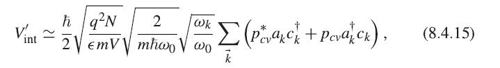
In Section 7.5.3 we defined the exciton creation operator c†k and the exciton– photon interactionwhere ak is the photon operator, and the constants in front of the sum are defined in Section 7.5.3.Suppose that excitons exist in a semiconductor with energy gap h̄ω0 and exciton binding energy
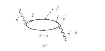
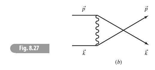
Write down the integral for the diagram shown in Figure 8.7(b). i-p (b) K
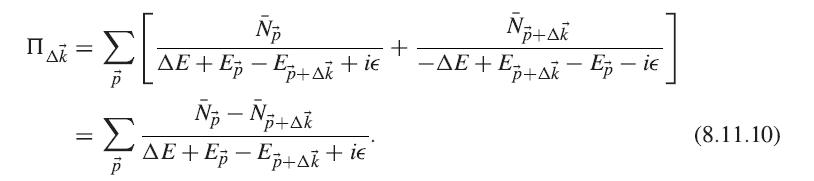
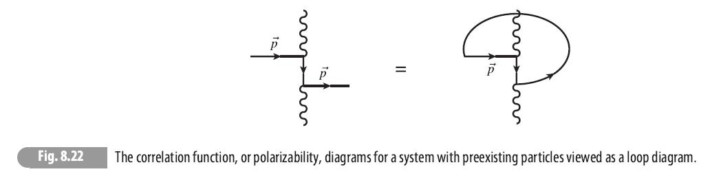
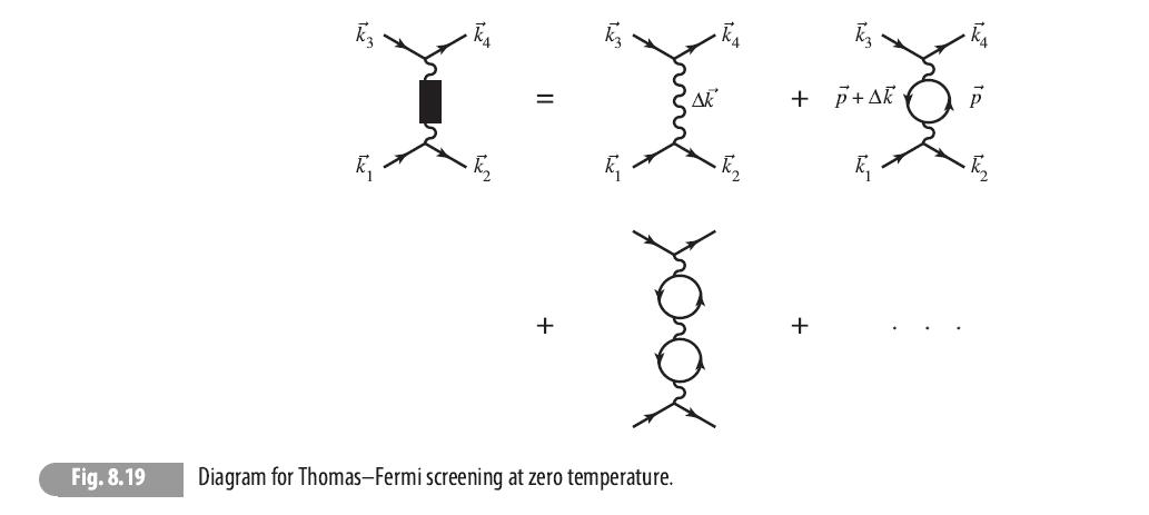
Use the finite-temperature propagators of Section 8.10 for fermions for the single-loop diagram shown in Figure 8.19, and show that you obtain the same Lindhard formula (8.11.10).Actually, a two-external-leg diagram can also be viewed as a loop, as illustrated in Figure 8.22, if we view the
Suppose that an initial state consists of two electrons with the same spin in states qvector)1 and q(vector)2, and the final state consists of electrons in states q(vector)3 and q(vector)4 Deduce the scattering matrix elements that are first and second order in the Coulomb interactionfollowing the
Verify Wick’s theorem explicitly for the case of four operators, namely two creation operators and two destruction operators for bosons in the same state k(vector). There are 4! = 24 possible time orderings, but just pick two possible orderings to verify.
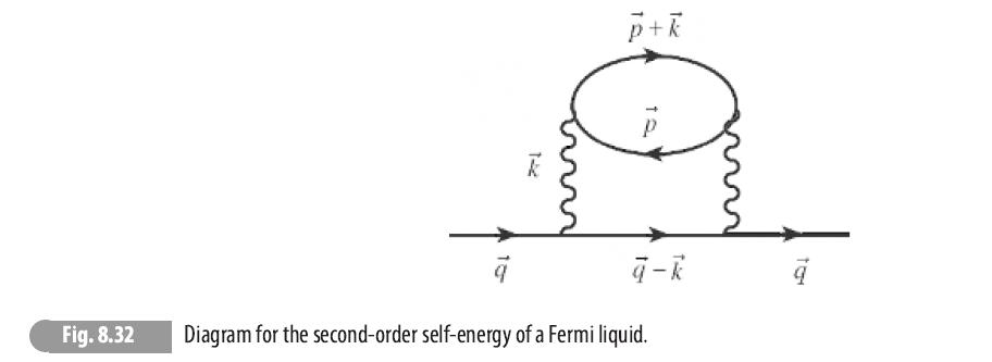
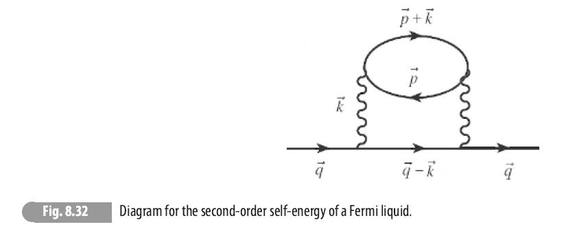
Use the finite-temperature Green’s functions method of this section to compute the diagram shown in Figure 8.32, used in the Fermi liquid theory at the end of this chapter. Show that the result for the imaginary self-energy has the same two terms as in (8.15.17), which are also the same as the
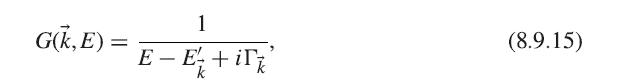
Prove that (8.9.16) is the Fourier transform of (8.9.15), when the integral over time is divided by h̄ to give units of inverse energy. G(k, E) = E - E₂+ir k (8.9.15)
Show that the Matsubara Green’s function is periodic, that is, forproveUse the cyclic property of traces (8.13.10), above. G(T₁ T₂) = -i(T(az(t₁)a/(t₂)))T, k
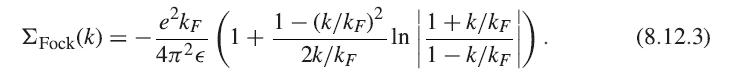
Show the consistency of the exchange energy formula (8.12.15) and the result of integrating (8.12.3). ΣFock(k) = - e²kF 4л²€ 1+ 1 - (k/kF)² 2k/kF -In 1+k/kF 1 - k/kF (). (8.12.3)
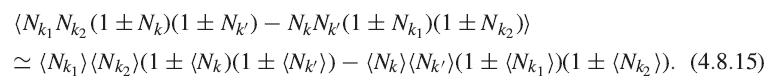
According to (4.8.15) in Section 4.8, the scattering rate for fermions is proportional to 1/2 (UD − UE)2, where UD is the direct interaction vertex and UE is the exchange vertex. In the diagram shown in Figure 8.32, only the direct term proportional to U2D occurs. Show that if you account for
Show that in the limit of a noninteracting gas, the spectral functionis proportional to AS (k, w)
Write down all the possible third-order Rayleigh–Schrödinger diagrams that have an initial state of a photon and a final state of an emitted phonon and a photon, for two electron bands c and v. If you apply a selection rule that phonons do not cause electrons to change bands, which diagrams are
Determine the k = 0 plasmon frequency for a gas of electrons with mass equal to the free electron mass, in a system with low-frequency dielectric constant ϵ = 2ϵ0, and density 1019 cm−3. A convenient unit conversion is e2/4πϵ0 = 1.44 × 10⁻⁷ eV-cm.
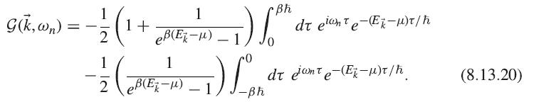
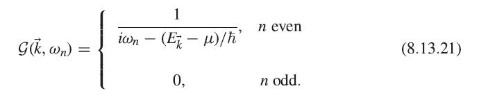
Verify that (8.13.21) follows from (8.13.20) for bosons, and derive the comparable relation for fermions. 1 Bh - / - ( 1 + 2M² - A) - 1) / ²² eß(E-μ) - G(k, wn) = − 1/2 (1 -=-2/2 (²3-10-1) Lp² eB(E-) dt elante-E-μ)t/h dt eant e-(E-μ)t/h (8.13.20)
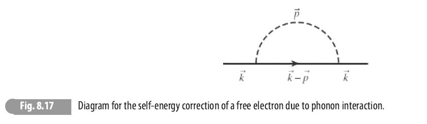
(a) Write down the Matsubara sum for the electron self-energy diagram for phonon interaction shown in Figure 8.17, and resolve the sum using the method of residues given here.(b) Using the identities of this section, show that you get the same answer as in Section 8.10 when using analytic
Determine the plasmon frequency to quadratic order in Δk, assuming an isotropic, Maxwell–Boltzmann distribution of electrons.
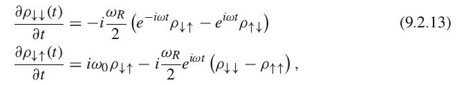
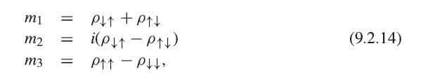
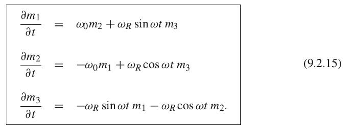
Show that the Bloch equations (9.2.15) and (9.2.19) follow from (9.2.13) and definitions (9.2.14) and (9.2.18). apud (1) Ət apy1(1) Ət @R 2 (e-iot = iwoP↓↑ - P↓↑ @R 2 - eiwt ptt) elot (P↓↓ - P↑↑), (9.2.13)
Equation (9.1.14) seems to contradict (9.1.4), since it has a minus sign. Equation (9.1.14) is an equation for the density matrix elements, however, while (9.1.4) is for the time-dependent operator. Show that these two equations both give the same result for the time evolution of the element ρmn =
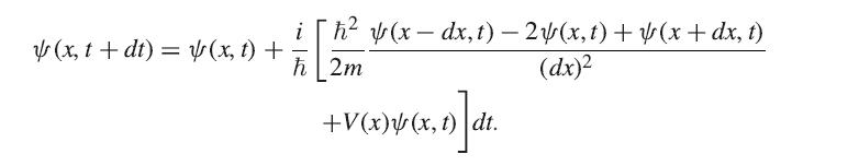
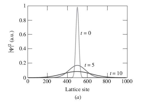
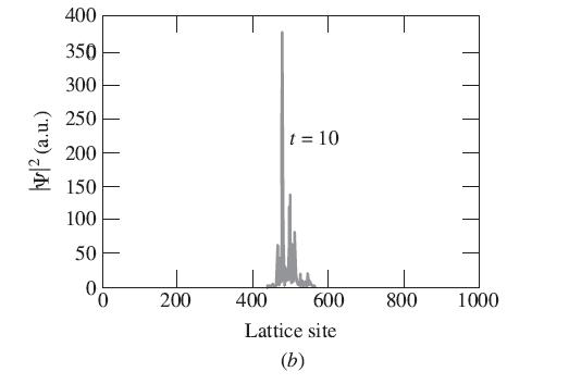
It is not hard, with modern computing power, to solve the time-dependent Schrödinger equation in one dimension using an iterative approach. We define the wave function ψ(x, t) on a set of discrete points x separated by distance dx, and update ψ(x, t) for a series of time steps dt according to
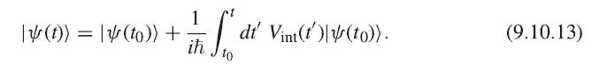
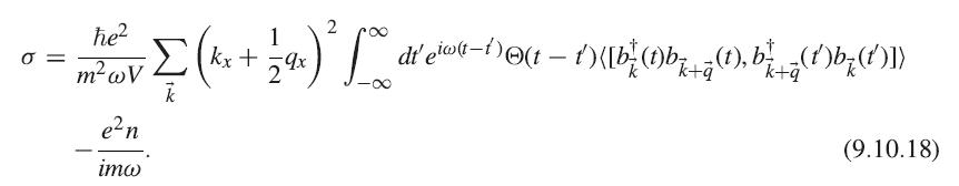
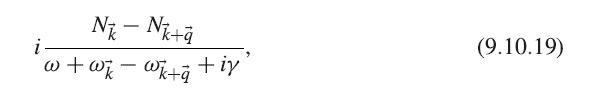
Prove, using the fermion anticommutator (8.6.13), that (9.10.19) is the result of the time integral in (9.10.18). |(t)) = √(to)) + Sat 1 ih to dt' Vint(t)\(to)). (9.10.13)
Calculate the average power of Johnson noise in watts in the frequency range 100–110 MHz at T = 300 K, in a circuit with R = 50 μ.
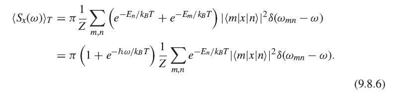
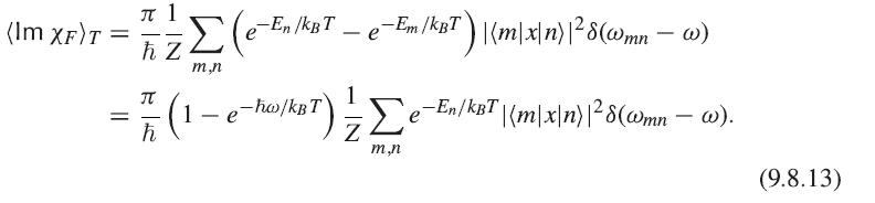
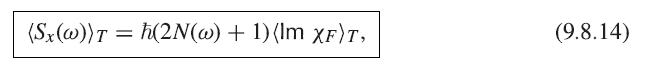
Show that the ratio of the thermal factors in (9.8.6) and (9.8.13) give the result (9.8.14). 1 (St(w)\r = π=Σ(e-En/kgT + e-Em/kBT) {{m\x|n)128(wmn - ω) = te m,n (1te-hio/kBT) /kBT) #Σ e-En/KAT –En/kBT|{m\x|n}|28(wmn - ω). =π]1 m,n (9.8.6)
Show, using the same approach as for thermal bosons, that thermal fermions have K(0) = 0.
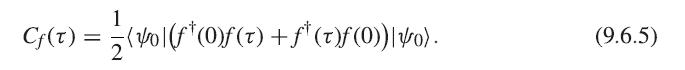
(a) The correlation functionused in (9.6.10) is not Hermitian. Show that if the correlation function is made Hermitian by the method used in (9.6.5), the spectral function will be symmetric with respect to ω = 0.(b) Find the spectral function for the case of a noninteracting boson gas, for a
A laser pulse has electric field proportional toand is repeated every period T0. Compute its correlation function, assuming T0 ≫ τ0, as well as its spectral density function (in arbitrary units), and its coherence length. e-iwote-(t-to)²/t2
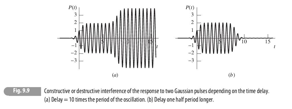
Use (9.4.2) to generate the response of a system to two pulses with Gaussian envelope functions, and create plots like those shown in Figure 9.9, using a program like Mathematica. To do this, you should first integrate the Gaussian pulse functionPlot the response of the system to several different
Calculate the Rabi frequency for a two-band semiconductor with gap energy 1.5 eV, excited by a cw laser with power 500 mW and beam width 1 mm, for an oscillator strength approximately equal to unity.For this laser characteristic, how long will a π-pulse be?
Prove the relation (9.2.10). Show that it is true for boson operators as well as fermion operators. [bb, bmbn ] = bmbn³nm-bmbn Sn.m. (9.2.10)
Show that the density operator in the mixed case still obeys the same normalization rule,Show that it still obeys the Liouville equation. Σpm = 1. n (9.1.17)
(a) Calculate the tadpole diagram for a zero-temperature Fermi gas using the Feynman method (treating the vacuum as the ground state of the Fermi sea) and show that this gives the same answer as the T = 0 limit of the Matsubara calculation given here. You will need to add a similar exponential
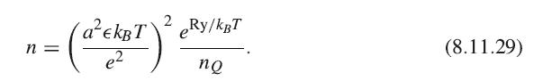
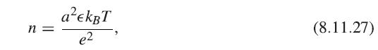
(a) Use a program like Mathematica to plot the phase boundary (8.11.29) in the n–T plane, for the ionization catastrophe, and also the phase boundary (8.11.27), for exciton radius a = 50 Å, exciton binding energy Δ = 10 meV, ϵ/ϵ0 = 10, and effective electron and hole masses both one-tenth the
Determine the Larmor frequency in hertz for a nucleus with spin- 1/2 and atomic mass number of 50, in a magnetic field of 10 T.
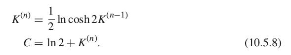
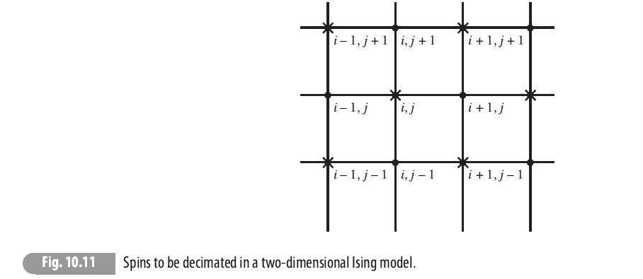
What is the renormalization rule for the two-dimensional decimation procedure illustrated in Figure 10.11, analogous to (10.5.8)? How many constants need to be introduced? K(n) 1 = In cosh 2K(n-1) C = ln 2+K(n) (10.5.8)
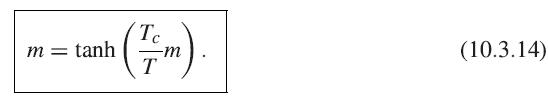
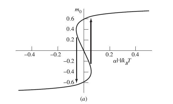
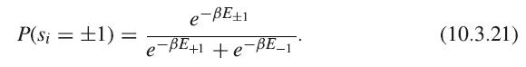
Show that near T = Tc, the solution (10.3.14) gives the same value of m0 as (10.4.3). m=tanh Te -m T (10.3.14)
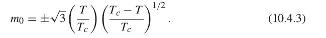
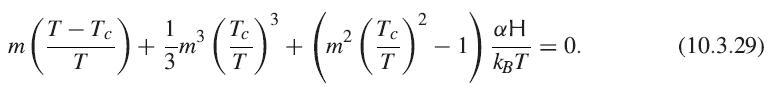
Use a program like Mathematica to plot the solutions m0 of (10.3.29) to generate a hysteresis curve like that shown in Figure 10.8. Plot the curve for a number of values of Tc/T and show how the system transforms as T moves through Tc. 3 2 T-Tc 1 aH 3 m „( ¯ ¯7² ) + ¦~* ( 7 )² + (~² ( ²7 )
Determine the speed of a magnon wave in the mean-field Ising model for a system at room temperature, with Curie temperature of 1000 K, and coordination number of 6.
(a) Compute the surface energy cost for a flat domain wall in three dimensions in the Ising model.(b) Suppose that an Ising system at low temperature has nearly all spins aligned up. An external magnetic field is then applied, so that the lowest-energy state corresponds to all spins aligned down.
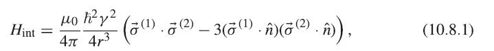
Using the lattice constant of iron r = 2.87 Å, and assuming the spins are parallel and aligned along the same axis, estimate J for the interaction (10.8.1). Then estimate the interaction J for iron using Tc = 2Jz/kB as defined in Section 10.3, assuming z = 8 for a bcc crystal, and knowing the
Use the estimate of the spin–orbit interaction energy at the beginning of Section 1.13 to estimate the strength of the Rashba term. First, show that the Rashba energy is of order (kaeff)〈HSO〉, where a = a0/Zeff is the effective Bohr radius of an atom and Zeff is defined in Section 1.13. Then
Compute the specific heat Cv = ∂U/∂T, with U = −∂Z/∂β = ∂(βF)/∂β, for the Ising model in the cases T < Tc and T > Tc and show that there is a discontinuity at Tc.
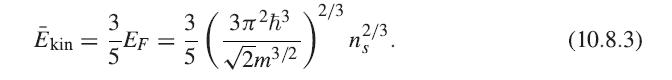
Show that (10.8.5) is correct by performing the average of the exchange energy (8.12.3) over all k. 2/3 3 3 Exin = ²-Er = ² ( 323/12) EF 5 5 n²/3. (10.8.3)
For T < Tc, we can write m(x(vector)) = m0 + δm, where m0 is the mean-field solution of the Ising model. Show that for h = 0, Gaussian fluctuations around the ordered state m0 lead to a divergent specific heat as T approaches Tc from below.
Fill in the missing mathematical steps from (10.8.20) to (10.8.23). In particular, show the counterintuitive result that Pauli exclusion can be ignored for the final state of the scattered electron. J = U² (2π)4 ckF Sª k² dk d (cos 0) kF k²dk'd(cos 0') ei(kR12 cos e-k'R 12 cos 0¹) Ek -
Using the same order-of-magnitude approximation as the previous exercise, estimate the typical coefficient β(k(vector)) that gives the fraction of opposite spin, according to (10.9.6). Assume that the nearby state mixed in is about 0.1 eV away, and take the other parameters from the previous
In deriving the interaction Hamiltonian for a free electron scattering from a localized electron, we showed that momentum conservation does not hold in the scattering process, and therefore an extra sum must be performed over all possible outgoing momenta. Show, following the same procedure as used
It is worthwhile to consider to what degree it is valid to treat different scattering processes in a single resistor as a series circuit of resistors. Consider a standard resistor in which the electrons have two main scattering processes: Scattering with defects, and scattering with crystal
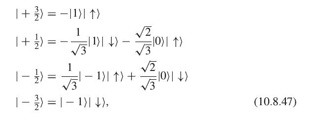
In the semiconductor GaAs, the valence band states at zone center are split by spin–orbit interaction into four degenerate stateswhere the states |1〉, |0〉, and | − 1〉 are the Bloch spatial cell functions with p-symmetry, and | ↓〉 and | ↑〉 are the pure spin states. The spin- 3/2
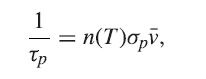
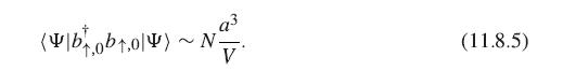
Show explicitly that (11.8.5) is correct for an arbitrary number N of pairs. ~Na³ V N~ (0+q⁰+qm) (11.8.5)
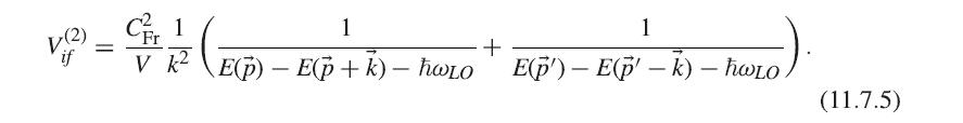
(a) What are the diagrams that you would write down in the Rayleigh– Schrödinger diagrammatic method that correspond to the two terms in (11.7.5)?(b) What are the diagrams you would write down in the Feynman method for the screening of the phonon-mediated Cooper pairing interaction? 1 1 =
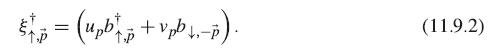
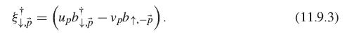
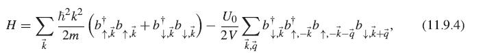
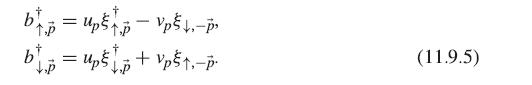
Prove that the operators (11.9.2) and (11.9.3) obey the fermion anticommutation rules. * = ( + ) داوران (11.9.2)
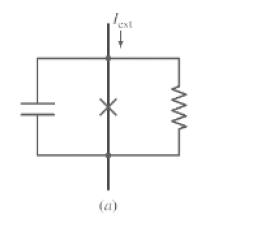
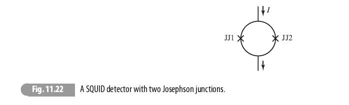
Equation (11.11.13) was deduced neglecting the associated parallel resistance of the junctions, which shown in Figure 11.23(a). Rewrite this equation for the case in which each junction has a parallel resistance R, and determine the maximum voltage drop ±V across the SQUID shown in Figure 11.22
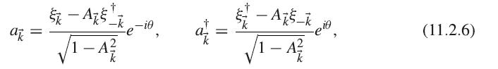
Verify by direct substitution in the Hamiltonian (11.2.4) that the definition of A(vector)k given in (11.2.6) will eliminate the off-diagonal terms. ak † -A75-10 √1-A² || حمد - As-k √1-A² (11.2.6)
Verify the calculation that the London penetration depth in a realistic superconductor is very small, using the electron density n0 = 1020 cm−3 and the mass and charge of an electron in vacuum (which is, of course, an approximation since electrons in a solid can have mass different from
What density of two-level oscillators is implied by the assumption made above, namely A/ϵ0 ≪ 1, for ω in the visible optical range of the spectrum, oscillator strength of the order of unity, and spontaneous recombination time of a few picoseconds?
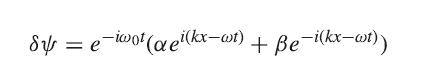
Show that linearizing the Gross–Pitaevskii equation leads to the Bogoliubov energy dispersion for excitations. To do this,(a) Write the wave function of the condensate as ψ0 +δψ, where ψ = √n0 e−iω0 t is the ground state wave function and δψ is a perturbation, and derive the
Typical values of the nonlinear interaction potential for excitons are U ∼10−11 meV-cm2. Convert this value to a photon–photon χ(3) value in units of m2/V2, using the formulas of Section 4.4 to convert electric field amplitude E to photon number density, and taking a typical solid state
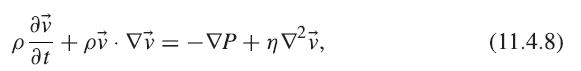
The Navier–Stokes equation governing the flow of an incompressible fluid is (see, e.g., Chaikin and Lubensky 1995: 449)where ρ is the mass density, v(vector) is the fluid velocity, P is the pressure, and η is the viscosity. Show that the requirement ∇ × g(vector) = 0 implies that the
Determine the critical number of particles for condensation at a fixed temperature in a three-dimensional harmonic potential with energy U = 1/2kr2. The quantum states in a harmonic potential are discrete, with energy where ω = √k/m and degeneracy g = (n + 1)(n + 2)/2, where n = 0, 1, 2, . . ..
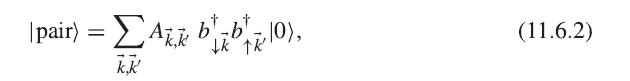
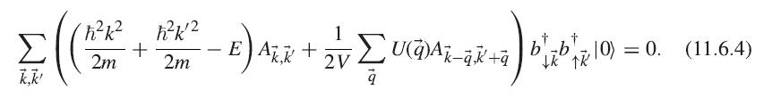
Show that (11.6.4) follows from (11.6.3), (11.6.2), and the fermion anticommutation relations. |pair) = ΣAkk bab|z|0), 10 k,k' (11.6.2)
Plot k2(A2k)/(1 − A2k) vs k assuming constant interaction vertex U, for various choices of U, to see what the distribution of excited particles looks like at T = 0.
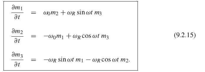
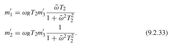
(a) Prove that (9.2.33) is the steady-state solution to (9.2.15), in the limit T1 ≫ T2. (b) Use a program like Mathematica to plot the magnitude of the Bloch vector as a function of ω̃, for several values of T2. am1 at дм2 at am3 Ət = wom2wR sin wt m3 = = -wom₁ + wR COS wt m3 -WR
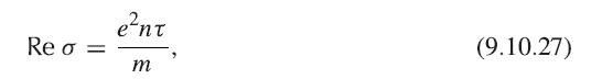
Prove the formula (9.10.27) by taking the real part of the conductivity. Re o = ent m (9.10.27)
Imagine doing a “two-slit interference” experiment with electrons that go through two separate tubes (with no inelastic dephasing), as illustrated in Figure 9.23. The source emits wave packets that are well defined in time, so that for a certain period of time, we can say that the wave packet
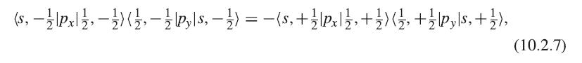
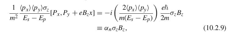
Prove the statements (10.2.7) and (10.2.8), and that the other terms vanish as stated, by explicitly evaluating the matrix elements, using the band functions in (1.13.9) and (1.13.10), and substituting Φx = x, Φy = y, Φz = z, and Φs = 1.Show also that the term αn is real for these states,
The Ising model can easily be solved numerically, if you are familiar with a basic programming language. Create an array or matrix si, i = 1, . . . , N, which can have value either 1 or −1. The initial values can be picked randomly. The array is updated by the following algorithm: (1) For
Estimate the magnetization field M(vector) generated by a solid with 1023 atoms per cubic centimeter, all with a single spin aligned in the same direction, and a g-factor of 2. If this is a ferromagnet, what B-field does it generate at its surface?
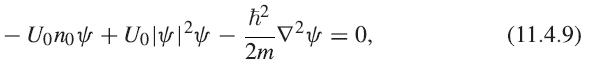
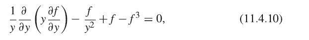
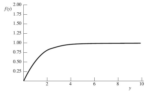
(a) The Ginzburg–Landau equation can be written aswhere n0 is the condensate density when ∇ψ = 0. Show that in the case of a straightline vortex with cylindrical symmetry, this can be written in unitless form aswhere y = r/r0, with r0 = h̄/√2mU0n0, and ψ = √n0eiθ f (r/r0). To do this,
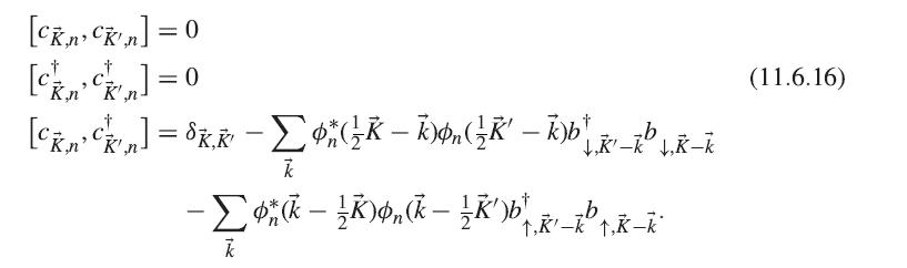
Prove the commutation relations (11.6.16), assuming that the wave function ϕn(k(vector)) is normalized and symmetric, that is ϕn(−k(vector)) = ϕn(k(vector)). [CKn, CK¹.n] =0 [ckckn] - - [Ckck] = $kk - Σøn (⁄K – K)øn(½K¹ − k)b¹¸k¹_k² ↓‚k-k = — K'n k = - - Σø*(k −
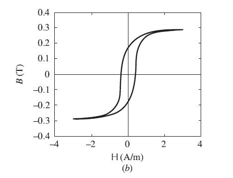
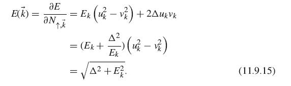
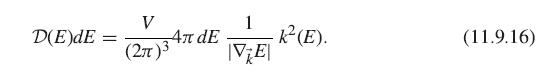
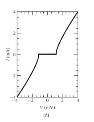
Compute the integral of the density of states (11.9.16) for the quasiparticle energy spectrum (11.9.15), and plot it (setting μ = 1 and Δ = 0.02, and all other constants to unity). It should have the same form as the experimental results for the normal–insulator–superconductor junction
Compute numerically and plot the universal curve Δ(T)/Δ(0) implied by (11.9.18). Ec 1 = D(EF) S Uo 2V dEk 2√² + E² tanh A² + E²/2kBT), (11.9.18)
What is the value of the critical field if a is 50 meV and the condensate density is 1022 cm−3? Is this obtainable by modern magnet systems?
Write down, but do not solve, the full equations for the dynamics of the phase jumps in the Josephson junctions of a SQUID in the presence of magnetic flux, using the model circuit given here. How are these equations altered if you include the self-inductance of the loop?
This analysis using the Bogoliubov model does not apply to liquid helium-4, because it is a strongly interacting system. Nevertheless, we can estimate the critical velocity for the superfluid by the following approximation:(a) The Born approximation, also known as the s-wave scattering
What is the critical current density, in amperes per cm2, of a superconductor with critical field of 15 T and London penetration depth of 0.5 μm?
What is the critical temperature for Bose–Einstein condensation of a gas of electron pairs at a density of 1022 cm−3, according to the ideal gas formula of Section 11.1, assuming that the electrons have the same effective mass as in vacuum? How does this Tc compare to typical superconductor Tc
Estimate the work needed to bring a superconductor with volume of 1 cm3 from infinity (where the magnetic field is zero) to a location with constant magnetic field equal to 1 tesla, assuming all magnetic flux is excluded from the superconductor.If a superconductor is placed in a uniform magnetic
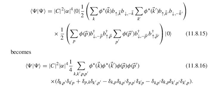
Show explicitly that the second-order term of the normalization condition (11.8.11) is correct, by showing thatShow that the last two terms with four δ-functions are negligible compared to the first two terms. **qtay Z) Flopolzhol = (mm) becomes τη X (ΣΣΕ) Ιω με τα
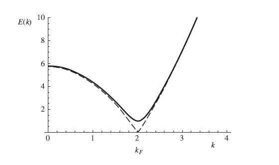
Show that substitution of the operators (11.9.5) into the Hamiltonian (11.9.4) gives the Hamiltonian (11.9.6). E(K) 10 8 6 4 2 0 1 2 KF 3 k
What is the sheet current density K (in units of amperes per cm) that will be generated on the surface of a cylindrical superconductor with radius 2 cm, according to (11.10.4), assuming all the current flows within one London penetration depth of the surface? Assume that the sheet current
(a) Determine the natural oscillation frequency of the phase difference Δθ across the Josephson junction equivalent circuit with I ext = 0, in the limit of low amplitude.(b) At what value of Iext will there be no local minima in the effective potential U(Δθ) at any value of Δθ?
Show that the operatorsobey boson commutation rules.
Showing 100 - 200
of 269
1
2
3
Step by Step Answers