New Semester
Started
Get
50% OFF
Study Help!
--h --m --s
Claim Now
Question Answers
Textbooks
Find textbooks, questions and answers
Oops, something went wrong!
Change your search query and then try again
S
Books
FREE
Study Help
Expert Questions
Accounting
General Management
Mathematics
Finance
Organizational Behaviour
Law
Physics
Operating System
Management Leadership
Sociology
Programming
Marketing
Database
Computer Network
Economics
Textbooks Solutions
Accounting
Managerial Accounting
Management Leadership
Cost Accounting
Statistics
Business Law
Corporate Finance
Finance
Economics
Auditing
Tutors
Online Tutors
Find a Tutor
Hire a Tutor
Become a Tutor
AI Tutor
AI Study Planner
NEW
Sell Books
Search
Search
Sign In
Register
study help
mathematics
statistics
Probability & Statistics For Engineers & Scientists 7th Edition Ronald E. Walpole, Raymond H. Myers, Sharon L. Myers, Keying - Solutions
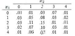
A delivery truck travels from point A to point B and back using the same route each clay there are four traffic lights on the route. Let Xi denote the number of red lights the truck encounters going from A to B and X2 denote the number encountered on the return trip. Data collected over a long
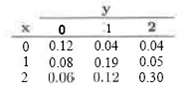
A convenience store has two separate locations in the store where customers can be: checked out as they leave. These locations both have: two cash registers and have two employees that check out customers. Let X be the number of cash registers being used at a particular time for location L and Y
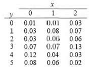
Consider a ferry that can carry both buses and cars on a trip across a waterway. Each trip costs the owner approximately 810. The fee for cars is $3 and the fee for buses is $8. Let X and Y denote the number of buses and cars, respectively, carried on a given trip. The joint distribution of X and V
As we shall illustrate in Chapter 12, statistical methods associated with linear and nonlinear models are very important. In fact, exponential functions are often used in a wide variety of scientific and engineering problems. Consider a model that is fit to a set of data involving measured values
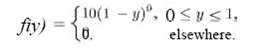
Consider Review Exercise 3.75. It involved Y, the proportion of impurities in a batch and the density function is given by? (a) Find the expected percentage of impurities. (b) Find the expected value of the proportion of quality material (i.e., find E (1 ? Y)). (c) Find the variance of the random
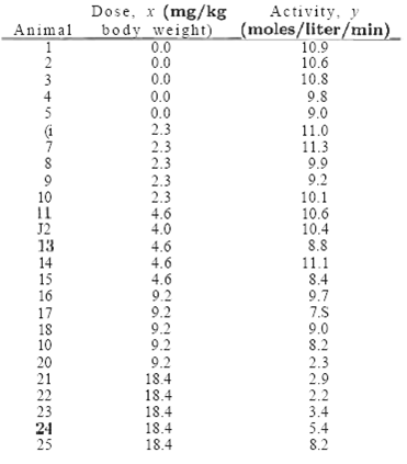
A study conducted at VP1&SU to determine if certain static arm-strength measures have an influence on the "dynamic lift" characteristics of an individual. Twenty-five individuals were subjected to strength tests and then were asked to perform a weight-lifting test in which weight was dynamically
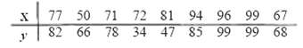
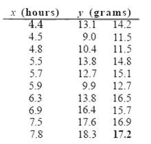
The grades of a class of 9 students on a midterm report (x) and on the final examination (y) are as follows(a) Estimate the linear regression line.(b) Estimate the final examination grade of a student who received a grade of 85 on the midtermreport.
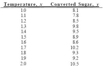
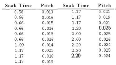
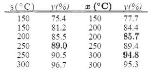
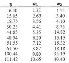
A study was made on the amount of converted sugar in a certain process at various temperatures. The data were coded and recorded as follows:(a) Estimate the linear regression line.(b) Estimate the mean amount of converted sugar produced when the coded temperature is 1.75.(c) Plot the residuals
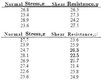
In a certain type of metal test specimen, the normal stress on a specimen is known to be functionally related to the shear resistance. The following is a set of coded experimental data on the two variables:(a) Estimate the regression line ? y?x = a + ? x.(b) Estimate the shear resistance for a
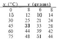
The amounts of a chemical compound y, which dissolved in 100 grams of water at various temperatures, .r, were recorded as follows:(a) Find the equation of the regression line.(b) Graph the line on a scatter diagram.(c) Estimate the amount of chemical that will dissolve in 100 grams of water at50?C.
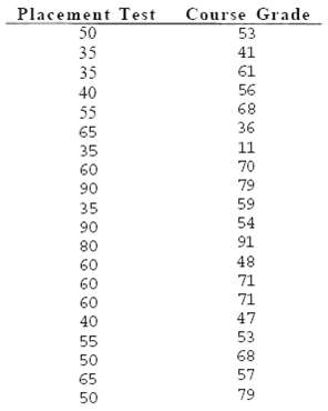
A mathematics placement test is given to all entering freshmen at a small college. A student who receives a grade below 35 is denied admission to the regular mathematics course and placed in a remedial class. The placement test scores and the final grades for 20 students who took the regular course
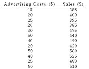
A study was made by a retail merchant to determine the relation between weekly advertising expenditures and sales. The following data were recorded:(a) Plot a scatter diagram.(b) Find the equation of the regression line to predict weekly sales from advertising expenditures.(c) Estimate the weekly
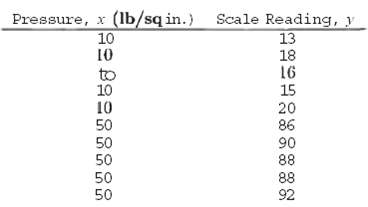
The following data were collected to determine the relationship between pressure and the corresponding scale reading for the purpose of calibration. (a) Find the equation of the regression line. (b) The purpose of calibration in this application is to estimate pressure from an observed scale
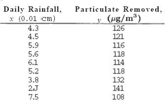
A study of the amount of rainfall and the quantity of air pollution removed produced the following data:(a) Find the equation of the regression line to predict, the particulate removed from the amount of daily rainfall.(b) Estimate the amount of particulate removed when the daily rainfall is x =
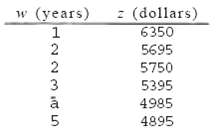
The following data are the selling prices z of a certain make and model of used car w years old. Fit a curve of the form ? z?w = ? ? w by means of the nonlinear sample regression equation z = c d w.
The thrust of an engine (y) is a function of exhaust temperature (x) in ?F when other important variables arc held constant. Consider the following data.(a) Plot the data.(b) Fit a simple linear regression to the data and plot the line through thedata.
A study was done to study the effect of ambient temperature x on the electric power consumed by a chemical plant, y. Other factors were held constant and the data were collected from an experimental pilot plant.(a) Plot the data.(b) Estimate the slope and intercept in a simple linear regression
The following is a portion of a classic data set called the "pilot plot data" in Fitting Equations to Data by Daniel and Wood, published in 1971. The response y is the acid content of material produced by titration whereas the regress or X is the organic acid content produced by extraction and
A professor in the School of Business in a university polled a dozen colleagues about the number of professional meetings professors attended in the past five years (X) and the number of papers submitted by those1 to refereed journals (Y) during the same period.The: summary data are given as
Assuming that, the ? i ?s are normal, independent with zero means and common variance ?2, show that A, the least squares estimator of ? in ? y?x = a + 0x, is normally distributed with mean a and variance
For a simple linear regression model where ? i ?s are independent and normally distributed with zero means and equal variances a~, show that, Y and have zero covariance.
With reference to Exercise 11.1, (a) Evaluate s2, (b) Test; the hypothesis that β = 0 against the alternative that β ≠ 0 at the 0.05 level of significance and interpret the resulting decision.
With reference to Exercise 11.2, (a) Evaluate s2; (b) Construct a 95% confidence interval for α; (c) Construct a 95% confidence interval for 0.
With reference to Exercise 11.3, (a) Evaluate s2; (b) Construct a 95% confidence interval for α; (c) Construct a 95% confidence interval for 3.
With reference to Exercise 11.4, (a) Evaluate s2; (b) Construct a 99% confidence interval for α; (c) Construct a 99%. Confidence interval for 3
With reference to Exercise 11.5, (a) Evaluate s2; (b) Construct a 99% confidence interval for α; (c) Construct a 99% confidence interval for 0.
Test the hypothesis that a = 10 in Exercise11.6 against the alternative that α < 10. Use a 0.05 level of significance.
Test the hypothesis that β = 6 in Exercise 11.7 against the alternative that β < 6. Use a 0.025 level of significance.
Using the value of s2 found in Exercise 11.18 (a), construct a 95% confidence interval for μ y׀85 in Exercise 11.2.
With reference to Exercise 11.4, use the value of s2 found in Exercise 11.20(a) to compute(a) A 95% confidence interval for the menu shear resistance when x = 24.5;(b) A 95% prediction interval for a single predicted value of the shear resistance when x = 24.5.
Using the value of s2 found in Exercise 11.19(a) graph the regression line and the 95% confidence bands for the mean response μ y׀x for the data of Exercise 11.3.
Using the value of s2 found in Exercise 11.19(a), construct a 95% confidence interval for the amount of converted sugar corresponding to x = 1.6 in Exercise 11.3.
With reference to Exercise 11.5, use the value of s2 found in Exercise 11.21(a) to compute(a) A 99% confidence interval for the average amount of chemical that will dissolve in 100 grams of water at 50° C;(b) A 99% prediction interval for the amount of chemical that will dissolve in 100 grams of
Consider the regression of mileage for certain automobiles, measured in miles per gallon (mpg) on their weight in pounds (wt). The data are from Consumer Reports (April 1997). Part of the SAS output from the procedure is shown in Figure.(a) Estimate the mileage for a vehicle weighing 4000
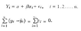
Show that in the case of a least, squares fit to the simple linear regression model
Consider the situation of Exercise 11.30 but suppose n = 2 (i.e., only two data points are available). Give an argument that the least squares regression line will result in (y1 — y1) = (y2 — y2) = 0. Also show that for this case R2 = 1.0.
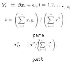
There are important applications in which due to known scientific constraints, the regression line must go through the origin (i.e., the intercept must be zero). In other words, the model should read, and only a simple parameter requires estimation. The model is often called the regression through
Given the data set (a) Plot the data. (b) Fit a regression line ''through the origin." (c) Plot the regression line on the graph with the data. (d) Give a general formula for (in terms of the y i and the slope b) the estimator of ?2. (e) Give a formula for V ar (y i); i = 1, 2. . . n for this
For the data in Exercise 11.33 find a 95% prediction interval at x = 25.
(a) Find the least squares estimate for the parameter β in the linear equation μ y׀x = 3x.(b) Estimate the regression line passing through the origin for the following data.
Suppose it is not known in Exercise 11.35 whether the true regression should pass through the origin. Estimate the linear model μ y׀x = a + β x and test the hypothesis that α = 0 at the 0.10 level of significance against the alternative that a ≠ 0.
Use an analysis-of-variance approach to test the hypothesis that 0 = 0 against the alternative hypothesis β ≠ 0 in Exercise 11.3 at the 0.05 level of significance.
Organophosphate (OP) compounds are used as pesticides. However, it is important to study their effect on species that are exposed to them. In the laboratory study, some Effects of Organophosphate Pesticides on Wildlife Species, by the Department of Fisheries and Wildlife at the Virginia Polytechnic
Test for linearity of regression in Exercise 11.5. Use a 0.05 level of significance. Comment
Test for linearity of regression in Exercise 11.6. Comment
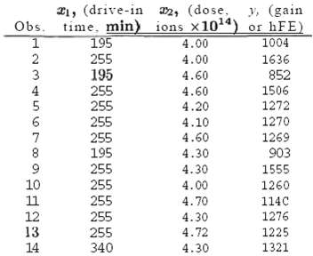
Transistor gain in an integrated circuit device between emitter and collector (hFE) is related to two variables [Myers and Montgomery (2002)] that can be controlled at the deposition process, emitter drive in time (SBI, in minutes), and emitter dose (x2, in ions x 1014). Fourteen samples were
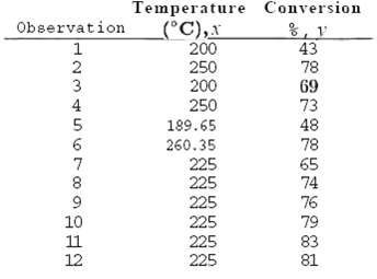
The following data are a result of an investigation as to the effect of reaction temperature x on percent conversion of a chemical process y. [See Myers and Montgomery (2002).] Fit a simple linear regression, and use a lack-of-fit test to determine if the model is adequate.Discuss.
Heat, treating is often used to carburize metal parts such as gears. The thickness of the carburized layer is considered an important feature of the gear, and it contributes to the overall reliability of the part. Because of the critical nature of this feature, a lab test is performed on each
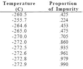
A regression model is desired relating temperature and the proportion of impurity from a solid substance passing through solid helium. Temperature is listed in degrees centigrade. The data are as presented here. (a) Fit a linear regression model. (b) Does it appear that the proportion of impurities
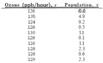
It is of interest to study the effect of population size in various cities in the United States on ozone concentrations. The data consist of the 1999 population in millions and the amount of ozone present per hour in ppb (parts per billion). The data are as follows:(a) Fit the linear regression
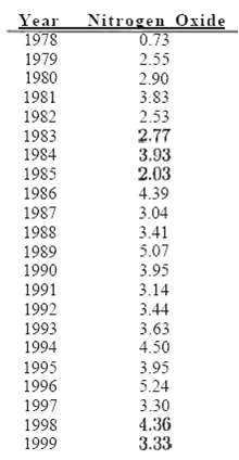
Evaluating nitrogen deposition from the atmosphere is a major role of The National Atmospheric Deposition Program (NADP, a partnership of many agencies). NADP is studying atmospheric deposition and the effect on agricultural crops, forest surface waters, and other resources. Nitrogen oxides may
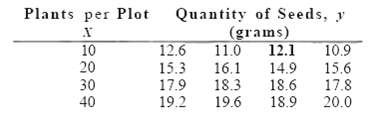
For a particular variety of plant, researchers wanted to develop a formula for predicting the quantity of seeds (grams) as a function of the density of plants. They conducted a study with four levels of the factor X, the number of plants per plot. Four replications were used for each level of X.
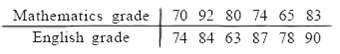
Compute and interpret the correlation coefficient for the following grades of 6 students selected atrandom:
Test the hypothesis that p = 0 in Exercise 11.49 against the alternative that p ≠ 0. Use a 0.05 level of significance.
Show the necessary steps in converting the equation r = b/a׀√S x x; to the equivalent form t = r√n-2/√1-r2
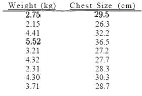
The following data were obtained in a study of the relationship between the weight and chest size of infants at birth: (a) Calculate r. (b) Test the null hypothesis that p = 0 against the alternative that p > 0 at the 0.0i level of significance. (c) What percentage of the variation in the infant
With reference to Exercise 11.1 assume that x and y is random variables with a bivariate normal distribution:(a) Calculate r.(b) Test the hypothesis that p = 0 against the alternative that p ≠ 0 at the 0.05 level of significance.
With reference to Exercise 11.9, assume a bivariate normal distribution for x and y.(a) Calculate r.(b) Test the null hypothesis that p = —0.5 against the alternative that p < —0.5 at the 0.025 level of significance.(c) Determine the percentage of the variation in the amount of particulate
With reference to Exercise 11.6, conclusions, construct(a) A 95% confidence interval for the average course grade of students who make a 35 on the placement test;(b) A 95% prediction interval for the course grade of a student who made a 35 on the placement test.
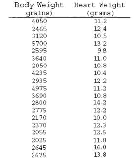
The Statistics Consulting Center at Virginia Polytechnic Institute and State University analyzed data on normal woodchucks for the Department of Veterinary Medicine. The variables of interest were bodyweight in grams and heart weight in grams. It was also of interest to develop a linear regression
The amounts of solids removed from a particular material when exposed to drying periods of different lengths are as shown. (a) Estimate the linear regression line. (b) Test at the 0.05 level of significance whether the linear model isadequate.
With reference to Exercise 11.7 construct(a) A 95% confidence interval for the average weekly sales when $45 is spent on advertising;(b) A 95% prediction interval for the weekly sales when 845 is spent on advertising.
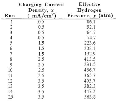
An experiment was designed for the Department of Materials Engineering at Virginia Polytechnic Institute and State University to study hydrogen embrittlement properties based on electrolytic hydrogen pressure measurements. The solution used was 0.1 N NaOH, the material being a certain type of
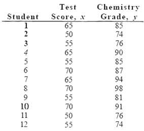
The following data represent the chemistry grades for a random sample of 12 freshmen at a certain college along with their scores on an intelligence test administered while they were still seniors in high school: (a) Compute and interpret the sample correlation coefficient. (b) State necessary
For the simple linear regression model, prove that E (s2) = a d.
The business section of the Washington Times in March of 1997 listed 21 different used computers and printers and their sale prices. Also listed was the average hover bid. Partial results from the regression analysis using SAS software are shown in Figure.(a) Explain the difference between the
Consider the vehicle data in Figure from Consumer Reports. Weight is in tons, mileage in miles per gallon, and drive ratio is also indicated. A regression model was fitted relating weight x to mileage y. A partial SAS printout in Figure shows some of the results of that regression analysis and
Observations on the yield of a chemical reaction taken at various temperatures were recorded as follows: (a) Plot the data. (b) Does it appear from the plot as if the relationship is linear? (c) Fit a simple linear regression and test for lack of fit. (d) Draw conclusions based on your result in(c).
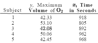
Physical fitness testing is an important as aspect of athletic training. A common measure of the magnitude of cardiovascular fitness is the maximum volume of oxygen uptake during a strenuous exercise. A study was conducted on 24 middle aged men to study the influence of the time it takes to
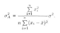
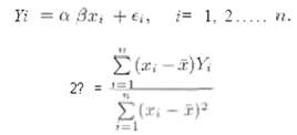
Suppose the scientist postulates a model Yi = a + β x i + ε i, i — \,2... n, and α is a known value, not necessarily zero.(a) What is the appropriate least squares estimator of β Justify your answer?(b) What is the variance of the slope estimator?
In Exercise 11.30, the student n was required to show that below, standard simple linear regression model. Does the same hold for a model with zero intercept? Show why or whynot.
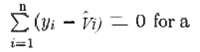
Suppose in Review Exercise 11.60 that we are also given the number of class periods missed by the 12 students taking the chemistry course. The complete data are shown next. (a) Fit a multiple linear regression equation of the form y = b a + b1x1 + b2x2. (b) Estimate the chemistry grade: for a
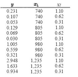
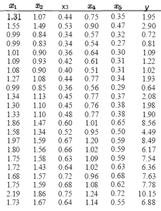
In Applied Spectroscopy, the infrared reflectance spectra properties of a viscous liquid used in the electronics industry as a lubricant were studied. The designed experiment consisted of the effect of band frequency x1 and film thickness x2 on optical density y using a Perkin-Elmer Model 621
A set of experimental runs was made to determine a way of predicting cooking time y at various levels of oven width x1, and flue temperature x2. The coded data were recorded as follows. Estimate the multiple linear regression equation ? Y?x1, x2 = ?0 + ?1x1 + ?2x2.
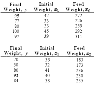
An experiment was conducted to determine if the weight of an animal can be predicted after a given period of time on the basis of the initial weight of the animal and the amount of feed that was eaten. The following data, measured in kilograms, were recorded:(a) Fit a multiple regression equation
(a) Fit a multiple regression equation of the form μ Y׀x = β0 + β1x1 + β2x2 to the data of Example 11.8.(b) Estimate the yield of the chemical reaction for a temperature of 225° C.
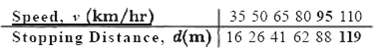
An experiment was conducted on a new model of a particular make of an automobile to determine the stopping distance at various speeds. The following data were recorded. (a) Fit a multiple regression curve of the form ? D?v = ?0 + ?1v + ?2v2. (b) Estimate the stopping distance when the car is
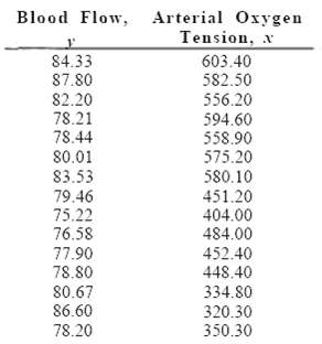
An experiment was conducted in order to determine if cerebral blood flow in human beings can be predicted from arterial oxygen tension (millimeters of mercury). Fifteen patients were used in the study and the following data were observed. Estimate the quadratic regression equation ? Y?x = 3o + ?1 x
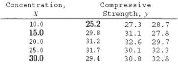
The following is a set of coded experimental data on the compressive strength of a particular alloy at various values of the concentration of some additive: (a) Estimate the quadratic regression equation ? Y?x = ?0 + ?1x + ?2x2 (b) Test for lack of fit of the model.
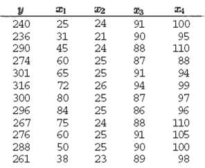
The electric power consumed each month by a chemical plant is thought to be related to the average ambient temperature x1, the number of days in the month x2, the average product purity x3, and the tons of product produced x4. The past year's historical data are available and are presented in the
The electric power consumed each month by a chemical plant is thought to be related to the average ambient temperature x1, the number of days in the month x2, the average product purity x3, and the tons of product produced x4. The past year's historical data are available and are presented in the
The personnel department of a certain industrial firm used 12 subjects in a study to determine the relationship between job performance rating (y) and scores of four tests. The data are as follows: Estimate the regression coefficients in the model y = bo + b1x1 + b2x2 + b3x3 + b4x4.
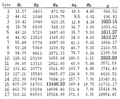
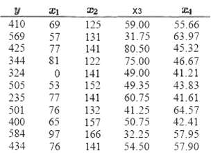
The following data reflect information taken from 17 U.S. Naval hospitals at various sites around the world. The regressors are workload variables, that is, items that result in the need for personnel in a hospital installation. A brief description of the variables is as follows:y = monthly
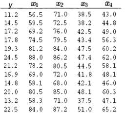
An experiment was conducted to study the size of squid eaten by sharks and tuna. The regressor variables are characteristics of the beak or mouth of the squid. The regressor variables and response considered for the study arex 1 = rostral length, in inches,x 2 = wing length, in inches,x 3 = rostral
Twenty-three student teachers took part in an evaluation program designed to measure teacher effectiveness and determine what factors are important. Eleven female instructors took part. The response measure was a quantitative evaluation made on the cooperating teacher. The regressor variables were
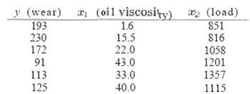
A study was performed on wear of a bearing y and its relationship to x1 = oil viscosity and x2 = load. The following data were obtained. [Prom Response Surface Methodology, Myers and Montgomery (2002)] (a) Estimate the unknown parameters of the multiple linear regression equation ? Y?x1,x 2 = 00 +
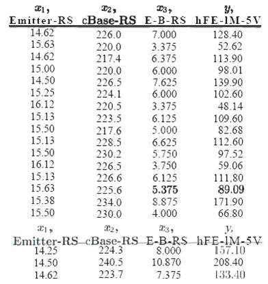
An engineer at a semiconductor company wants to model the relationship between the device gain and hFE(y) and three parameters: emitter-RS (x1), base-RS (x2), and emitter-to-base-RS (x3). The data are shown below: (a) Fit a multiple linear regression to the data. (b) Predict hFE when x1 = 14, x 2 =
For the data of Exercise 12.2, estimate a2.
For the data of Exercise 12.3, estimate a2.
For the data of Exercise 12.9, estimate a2.
Obtain estimates of the variances and the covariance of the estimator’s b1 and b2 of Exercise 12.2 on
Referring to Exercise 12.9 find the estimate of (a) σ2 b2. (b) Cov (b1 ‘64).
Using the data of Exercise 12.2 and the estimate of a2 from the exercise 12.17, compute 95% confidence intervals for the predicted response and the mean response when x1 = 900 and x2 = 1.00.
For Exercise 12.8, construct a 90% confidence interval for the mean compressive strength when the concentration is x = 19.5 and a quadratic model is used
Using the data of Exercise 12.9 and the estimate of a2 from Exercise 12.19 compute, 95% confidence intervals for the predicted response and the mean response when x1 = 75, x2 = 24, x3 = 90, and x4 = 98. Show calculations.
For the model of Exercise 12.7, test the hypothesis that β2 = 0 at the 0.05 level of significance against the alternative that β2 ≠ 0.
For the model of Exercise 12.2, test the hypothesis that β 1 = 0 at the 0.05 level of significance against the alternative that β1 ≠ 0,
For the model Exercise 12.3, test the hypothesis that β1 = 2 against the alternative that β1 ≠ 2? Use a P-value in your conclusion.
Consider the following data that is listed in Exercise 12.15. (a) Estimate ?2 using multiple regression of y on x1 and x2. (b) Compute predicted values, a 95% confidence; inter value for mean wear, and a 95% prediction interval for observed wear if x1?= 2 and x2 = 1000.
Showing 1900 - 2000
of 88243
First
13
14
15
16
17
18
19
20
21
22
23
24
25
26
27
Last
Step by Step Answers