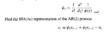
Question Answers
Textbooks
Search Textbook questions, tutors and Books
Oops, something went wrong!
Change your search query and then try again
Toggle navigation
FREE Trial
S
Books
FREE
Hire a Tutor
AI Tutor
New
AI Flashcards
FREE
Search
Search
Sign In
Register
study help
business
econometric analysis
Questions and Answers of
Econometric Analysis
(Lagged Dependent Variable) Generalize the score test for autocorrelation in Exercise 20.26 to the alternative hypothesis that [s,) is an AR(p) process instead of an AR(1).
[MA(1)] Find an analogue to Hatanaka's estimator (p. 512) for e in y=x8o+e, when, conditional on (x,), (,) is an MA(1) process instead of an AR(1) process.
(Unit Circle) In Example 25.2 we find the conditions for AR(2) stationarity. Lemma 25.2[AR(p) Covariance Stationarity, p. 655] gives an alternative approach: the routs ofmust lic strictly inside the
(Common Factor Test) Consider the regression model
[MA(1)] Show that F* | -1 -2] does not have a convergent set of coefficients for an MA(1) with a unit root.
(ARMA) Show that the sum of two AR(1) time series has an ARMA(2, 1) representation.
(Inversion) Show that the coefficients of the MA inversion of the AR(p) process (L), = u, can be found by the Taylor series formula (Theorem D.18). Id 1 s! de (z) -=0 Find the MA(00) representation
[MA(1)] Suppose that (e) is an MA(1) process. Show that the correlation between 8, and 8, -1 bounded in absolute value by one-half. is
|MA(1) Apply the Kalman filter to an MA(1) process. Confirm your results with Example 25.8.
[MA(q)] Suggest a reparameterization of the MA(g) specification that provides a way to constrain the roots of the associated characteristic equation to the unit circle. (HINT: cos i sin 9 are
(Score Test) In Section 25.7.4 of the Mathematical Notes, we show that the score tests for no autocorrelation in normally distributed disturbance terms are identical in the AR(p) and MA(p)
(NLS) Consider the NLS estimator described in (25.6)-(25.7). Show that BNLS and NLS are asymp totically independently distributed provided that x, does not include lagged dependent explanatory
[AR(p) Score Test] Consider the pth-order autoregressive model with the conditional log-likelihood function (25.8) and the null hypothesis of no serial correlation, 0. Show that one score test
(Projection) Reconsider the panel data model in (24.42) and (24.44) with the additional moment restrictions in Section 24.8. Bhargava and Sargan (1983) and Breusch et al. (1989) suggest assuming also
(IV) Consider generalizing Chamberlain (1982) to instrumental variables estimation. Suppose thatand that $X_{nt}$ contains elements that are correlated with $\epsilon_{nt}$ as well as $\alpha_{n}$.
Show that errors in variables can be overcome in a panel setting.
Derive the score test statisticfor $\sigma_{\alpha}^{2} = 0$ in the random-effects model [(24.9)-(24.11)]. The log-likelihood function permits $\sigma_{\alpha}^{2} S= N VarNITE[]} 2(7-1) VarNTInt] }
(Partitioned OLS) One can estimate the coefficients of the LSDV model with two steps: (1) take deviations from individual means and (2) fit these deviations with OLS. Extend this method to a model
(ML) Find the log-likelihood function for the random-effects panel data model, assuming that the latent variables are multivariate normal. Compare the MLE with the estimators discussed in this
(Linear Projection) The unrestricted estimation of the variance matrix (24.47) in Chamberlain's min- imum distance estimator may be a liability in small samples if the population variance is
(Hausman Test) Within the model of Chamberlain (1982) in Section 24.7, explain how to compute a Hausman specification test for Elez, IX) = 0 from the difference between the fitted coefficients from
(MD) Reconsider the two-step restricted MD estimator in (24.48). Alternatively, one can reduce the dimension of the first step of estimation by imposing &-0 at that stage as well. (a) Describe the
(Unbalanced Panel Data) In many panel data sets, the number of time periods available for each individual varies. (a) Describe the LSDV estimator for such cases. (b) Describe also the random-effects
(Dynamic Models) The dynamic panel data model begins with (24.27), which is analogous to the static specification (24.7). We might also assume thatby analogy with (24.8). Show that these two
(Hausman Test) Reconsider the Hausman specification test for the random-effects model (24.9)--(24.11).(a) Construct a Hausman specification test statistic using the difference between the OLS and
Suggest a consistent estimator for the asymptotic variance of the LSDV estimator even if there is conditional heteroskedasticity and covariance across the observations of each individual over time.
(OLS versus GLS) Let E[$\textbf{y}$|$\textbf{X}$] = $\textbf{X}\beta_0$. Ifthe dependent data are conditionally equicorrelated. Show that if a constant is one of the explanatory variables then OLS
(Feasible GLS) The estimators of variances in (24.23)--(24.24) contain an implicit estimator of $$\sigma_v^2$$.(a) What is this estimator?(b) Show that this estimator can be negative.(c) What would a
(Equicorrelation) Consider estimation of the parameters of the equicorrelated variance matrix $\Omega_0 =$$\sigma_u^2[[(1 - ho_0)I_T + ho_01_T1_T^T]$ given an observed vector y with $E[y] = 0$ and
(OLS) Consider the OLS estimator of $E[y_{n1}|X_1 = x_n^T\beta_0 + \alpha_0$ given that $y_{nt} = x_{nt}^T\beta_0 + u_{n} + \epsilon_{nt}$ and(24.10)-(24.11) hold.(a) What does the sample variance of
(LSDV) Show that the OLS estimator is a matrix-weighted average of the LSDV and between-groups estimators, $\hat{\beta}_{DV}$ and $\hat{\beta}_B$, respectively.
(LSDV) Show that, for $N \to \infty$ and $T$ fixed, $\hat{\beta}_{0DV}$ is a consistent estimator of $\beta_0$ but the $\hat{\alpha}_{n}$,$n = 1, \dots, N$, are not consistent estimators of the
(LSDV) Show that when $T=2$ the LSDV estimator of $\beta_0$ in (24.1) is equivalent to OLS fitted coefficients from a regression of $y_{n2} - y_{n1}$ on $x_{n2} - x_{n1}$.
(Hausman test) Suggest a gradient version of the Hausman specification test.
(Two-Step and MD) One can apply the minimum distance method to the two-step estimation framework described in Proposition 19 (Two-Step Asymptotic Variance, p. 507). Consider the two-step estimator
Using MD, find a more efficient restricted estimator than $$\hat{\theta}_{RN}$$ in (22.57) when $$C_N e \hat{A}_N^{-1}$$. Show that a test statistic based on the squared generalized distance between
(Linearized MD) Find a linearized MD estimator given restrictions of the form $$\theta_0 = s(\gamma_0)$$.
(Hausman Test) The variance matrix difference (22.26) excited many people when it was first published by Hausman because it made the computation of the variance estimator for a difference in
(MD) Describe a relatively efficient MD estimator based on the two-step estimator of the dynamic regression model given in Exercise 20.27.
(MD) Consider estimation of the coefficients of the MMSE linear predictor of $y_n$ given ($x_{n2}$, $x_{n3}$),Suppose that $E[y_n | x_n]$ is not linear and $Var[y_n | x_n]$ is not constant but that
(Normality Test) Use Theorem D.8 (Normal Distribution. p. 887) to show that the variance matrix of the moments in Example 22.5 is o Exx 0 0 30 E[x] 0 20+ 0 120 Ao = 30% E[x] 0 0 150 0 120 0 960 Show
(Minimum Chi-Square) Find analogous relationships to (22.47)-(22.49) between the OLS and RLS estimators. Also find the analogue to (22.38).
(Hausman Test) Show that the coefficients in the Hausman specification test regression on p. 580 are identical to the unrestricted estimates.
(Pretest Estimation) One might use the Hausman specification test to choose between two estimators based on different sets of moment restrictions. Describe the properties of such an estimation
(Simultaneous Equations) Reconsider the market model of Example 20.2(Simultaneous Equations, p. 492). GMM and the moment equations(a) Given that the 2SLS estimator is consistent and asymptotically
(Instrumental Variables) Find a way to compute the GMM test in Example 22.3 as the difference in OLS sums of squared residuals.
[Breusch-Godfrey AR Test] Consider the moment functions of the regression model with AR disturbances:where $v_t = \epsilon_t - ho \epsilon_{t-1}$ and $\epsilon_t = y_t - x_t'\beta$. Suppose that
Use a simple example to illustrate that the DD test fails to have a limiting chi-square distribution if$C_0 e A_0^{-1}$ even though $Col(C_0G_0) = Col(A_0^{-1}G_0)$ so that estimation is relatively
What are the consequences for the GMM hypothesis test if one uses a $C_N$ that does not produce a relatively efficient GMM estimator?
Explain the absence of the multiplicative factor 2 in the DD when one compares this test statistic with the LR test statistic.
Produce an illustration like Figure 17.3 for the GMM test statistics, including a representation of the MC test statistic.
(Errors in Variables) Reconsider the model of errors in explanatory variables in Example 20.1. Assume that the variables x, U. and an arc i.i.d. from a joint distribution with finite first and second
(IV and GMM) Describe how the assumptions supporting the IV estimator, Assumption 20.1(Latent Variable Model, p. 499), Assumption 20.2(Instruments, p. 499), and Assumption 20.3, (Convergence, p. 500)
Researchers use (20.31) to anticipate the direction of bias or inconsistency in OLS.(a) What would Campbell and Mankiw (1989) expect the bias to be in the OLS estimator of$$\beta_{02}$$ in (21.2),(b)
Campbell and Mankiw (1989) considered lagged first differences in income and in consumption separately as instrumental variables. Comment.
Hall (1978) also suggests (but does not estimate) a model with the constant-relative-risk-aversion utility function $$U(C) = C^{\gamma}/\gamma$$.(a) What is the Euler equation for such a model?(b)
(Two-Step Estimation) In Example 20.5, we noted that OLS with the LHS variable $y_t$ and the RHS variables $x_t$ and $x_{t-1}$ will deliver consistent estimators of $\beta_{01}$, $\beta_{02} +
(Score Test for Serial Correlation) In the dynamic regression (20.8) with autoregressive disturbances(20.1), if there is no autocorrelation in {$\epsilon_t$} ($\phi_1 = 0$), then the OLS estimator
(Orthogonality) The covariance matrix between $x_t$ and $z_t$ isbut orthogonality concerns whether $E[x_tz_t]$ equals zero. Explain why "correlation" is an appropriate term for discussing possible
(Heteroskedasticity and IV) Suppose that $(y_n, x_n, z_n)$ are i.i.d. such that$n = 1, \dots, N$. Let the number of instrumental variables in $z_n$ equal the number of explanatory variables in $x_n$.
(MMSE and IV) Under the conditions of Proposition 18, show that the probability limit of the IV estimator is the solution to the MMSE linear prediction problemwhere $\mu_γ(Z_n)$ and $\mu_γ(Z_n)$
(2SLS) Suppose that the number of variables (columns) in W equals the number of explanatory variables (columns) in X, in (20.50) for $\hat{\beta}_{2SLS}$.(a) Under what circumstances would this
(2SLS) Describe the 2SLS estimator for the demand equation (20.23) in Example 20.2. Be sure to include any additional assumptions that you require.
(2SLS) Show that we can compute the 2SLS estimator of the supply equation (20.50) by replacing $p_w$ with its OLS fitted value $w_p$, and running OLS. Will the OLS estimator of the sampling variance
(Projection and IV) Let us denote the IV estimator by $$ \hat{\beta}_{IV} = (W'X)^{-1}W'y $$.(a) Describe the IV fitted vector $$ X\hat{\beta}_{IV} $$ in terms of projection.(b) Compare the IV
We occasionally hear the remark that excluding an explanatory variable from a linear regression may result in misestimation of the slope coefficients whereas including an "irrelevant" explanatory
Give counterexamples to the following claims:(a) "Although errors in the explanatory variables cause inconsistency in the OLS estimator, errors in the dependent variable do not."(b) "Including an
Reestimate the Phillips curve for the model described in Section 20.1. Is the hypothesis ag = supported by the estimates?
(GNR) Section 19.6.1 notes that NLS can be used to compute an estimator that is asymptotically equivalent to the MLE for normal linear regression with AR autocorrelation. Describe the application of
(LMLE) Section 19.6.1 reviews several methods for computing estimators that are asymptotically equivalent to the MLE for normal linear regression with AR autocorrelation. Propose a two-step estimator
Derive an asymptotic approximation to the distribution of the first-order sample correlation among the OLS fitted residuals under the AR model for serial correlation.
(OLS versus GLS) If the OLS and GLS coefficient estimators are identical, can one use the estimated sampling variance matrix from OLS software for inferences about the population values of the
(Autocorrelation Function) Compute an estimate of the autocorrelation function up to 7 lags for the AR model for serial correlation using the estimate $\hat{\phi}$ = -0.498 reported in (19.3) and
(Score Test) Let the conditional log-likelihood of y given X be (19.11). Noting that(a) show that the OLS F test for φ0 = 0 in the artificial specificationis asymptotically equivalent to the
[AR Restrictions] According to (19.20), the AR model for serial correlation places nonlinear restrictions on the coefficients of E[yt|yt-1]. Describe a test of these restrictions. Suggest some
(Liapounov CLT) Proposition 15 (Asymptotic Distribution of OLS, p. 257) assumes that the $x_n$, ($n = 1, \dots, N$) are i.i.d. Suppose instead that the $x_n$ are deterministic such thatwhere D is a
(Nonlinear Least Squares) Reconsider the NLS estimator of Exercise 16.13. Suppose that $\{(y_n, X_n, Z_n), n = 1, \dots, N\}$ are i.i.d. random variables and that the conditional distribution of
(Two-Step Estimation) Suppose that $E[y_n | X_n] = X_n \beta_0$ and $Var(y_n | X_n) = \sigma^2_n (X_n \beta)^2$, so that the conditional variance of $y_n$ increases with the magnitude of its
(FGLS) Suppose that $E[y_n | x_n] = x_n'\beta_0$ and $Var(y_n | x_n) = (z_n'\gamma_0)^2$ where $|z_n'\gamma_0| > a > 0$ for all possible $z_n$ ($n = 1, \dots, N$). Also suppose that conditional
(Singular Variance) Suppose that the variance matrix $\Omega_0$ is singular. Show that the GLS estimator isprovided that $X'\Omega_0^{-1}X$ is nonsingular. (XX) X' y=argmin(y-X) (y-XB) B
(Recursive Residuals) How could one use the recursive residuals described in Exercises 8.15, 8.16, 9.9, and 10.9 to test the null hypothesis of homoskedasticity against the alternative in Example
(Relative Efficiency) Let E[y | X] = Xβ₀ and Var[y | X] = Ω₀ where β₀ ∈ ℝᵏ, X is full-row rank, and Ω₀ is nonsingular. Show that the RLS estimator βᵣ is not generally efficient
(Projection) According to (18.14), the GLS projector isShow that for any matrix A such that Col(AX) = Col(Ω₀⁻¹X) it follows that Pₓ₁AX = PₓΩ₀⁻¹X so that in general other weight
Let E[y|X] = Xβ₀ and Var[y|X] = Ω₀. Show that(Hint: Use the approach in Exercise 8.8.) F[s|X]= [[(I - Px)] N-K
(Restricted GLS) Show that the restricted GLS estimator, subject to the restriction Rβ₀ = r, is = BRGLS GLS (X','x) 'R'[RX'Q'x)-'R'](RGLS -r)
(Partitioned Fit) Find the generalized partitioned regression formula for the GLS estimator of E[y|X] = X₁β₁ + X₂β₂ where Var[y | X] = Ω₀.
(Eicker-White Variance Estimator) Explain why the presence of conditional heteroskedasticity in log-wages suggested by the score test (p. 418 and Example 18.4) implies that our test for equal
(OLS) Let E[y | X] = Xβ0 and Var[y | X] = Ω0 where β0 ∈ Rk, X is full-row rank, and Ω0 is nonsingular. Show that for all c ∈ Rk.directly from these expressions for the variance matrices.
(OLS) Let E[y | X] = Xβ0 and Var[y | X] = Ω0 where β0 ∈ Rk and X is full-row rank.(a) Find the conditional variance matrix of $ \hat{\beta}_{OLS} $ = Pxy given X.(b) Also find Var[y - $
(Testing on the Boundary) The Student distribution contains the normal as a special case, suggesting that one can construct hypothesis test statistics for normality with this generalization. Suppose
Argue that the test essentially examines whether the third- and fourth-moment restrictions of the normal distribution are satisfied.
(Score Test) Consider a score test for skewness based on the transformation in Exercise 13.13. What problem arises when the parameter $\alpha_2$ is unknown? Why does this problem disappear when one
(Generalized Inverse) Let the assumptions of Proposition 16 (ML Asymptotics, p. 320) hold. For restrictions $r(\theta_0) = 0$ such that $r_\theta(\theta_0)$ is full-row rank, show that(a)
(Score Test) In contrast to Example 17.9, follow Poirier et al. (1986) and use the power exponential family of distributions with p.d.f.to derive a score test of normality in the normal regression
(Minimum Chi-Square) Under the assumptions of Proposition 16 (ML Asymptotics, p. 320), prove that $E_{\theta}[N \cdot (\hat{\theta} - \theta - R\gamma(\theta))^T\gamma(\theta)(\hat{\theta} - \theta -
(Score Test) In (17.11), the score test statistic is S=N ENILOR (OR) EN [LO(OR)]
[C(α) Test] Explain the C(α) test for the restrictions θ2 = 0 on θ = [θ1', θ2']'.(a) Construct a generalization of C(α) for restrictions r(θ) = 0.(b) Show that C(α) ≥ 0 in (17.26). Is this
(Invariance) Suppose that θ ∈ R2 and consider testing the restriction θ1 = θ2 in the form θ1/θ2 = 1.(a) Reparameterize the likelihood function in terms of θ1 and y = θ1/θ2.(b) Find the
Using an example, show that the four classical test statistics are not necessarily asymptotically equivalent when the null hypothesis is false.
(Test Consistency) Following Proposition 17 (Classical Test Consistency, p. 402), we show that the Wald test is consistent. Prove that the LR, score, and C(α) tests are also consistent under the
Showing 1 - 100
of 618
1
2
3
4
5
6
7