New Semester
Started
Get
50% OFF
Study Help!
--h --m --s
Claim Now
Question Answers
Textbooks
Find textbooks, questions and answers
Oops, something went wrong!
Change your search query and then try again
S
Books
FREE
Study Help
Expert Questions
Accounting
General Management
Mathematics
Finance
Organizational Behaviour
Law
Physics
Operating System
Management Leadership
Sociology
Programming
Marketing
Database
Computer Network
Economics
Textbooks Solutions
Accounting
Managerial Accounting
Management Leadership
Cost Accounting
Statistics
Business Law
Corporate Finance
Finance
Economics
Auditing
Tutors
Online Tutors
Find a Tutor
Hire a Tutor
Become a Tutor
AI Tutor
AI Study Planner
NEW
Sell Books
Search
Search
Sign In
Register
study help
business
econometric analysis
An Introduction To Classical Econometric Theory 1st Edition Paul A. Ruud - Solutions
(Quadratic Approximation) Confirm the quadratic approximation in (17.21) using the following steps.(a) Write out a second-order Taylor series expansion for $E_\theta[L(\theta_B)]$ around $\theta = \theta_0$.(b) Use the argument in Section 15.3.2 to show that the Hessian in the expansion converges
(Convergence Criterion) Provide an interpretation of the computational convergence criterion(16.17) discussed in Section 16.5 in terms of hypothesis testing.
[C($\alpha$) Test] Add a representation of the C($\alpha$) test to Figure 17.3.
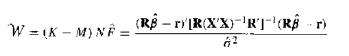
(F Test) Show that W for $H_0: R\beta = r$ in the normal linear regression model when the variance $\sigma^2$is unknown iswhere F is the F statistic in (11.1). W=(K-M) NR= (RB-r[R(XX) RT(RBT) r)
Let the assumptions of Proposition 16 (ML Asymptotics, p. 320) hold. Also, partition the parameter vector $\theta$ into $[\theta_1', \theta_2']'$ and suppose that $\theta_1$ and $\theta_2$ have the same dimensions. Write out the LR, S, and W test statistics for each of the following null
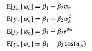
(LMLE) Show that the LMLE will work with any initial estimator that is $\sqrt{N}$ consistent under the conditions of Lemma 15.7(LMLE, p. 333).*16.13 Suppose that $\{(x_n, y_n), n = 1, \dots, N\}$ are i.i.d. random variables and that the conditional distribution of $y_n$ given $x_n$ is
(LMLE) Under the conditions of Lemma 15.7(LMLE, p. 333), show that an optimal step length for the given search direction also produces an estimator that is asymptotically equivalent to the MLE. (Such step lengths may improve the small sample performance of the LMLE.)
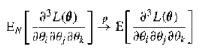
(LMLE) Suppose that the third derivatives of the log-likelihood function satisfy the uniform LLN(Lemma 15.1, p. 321) so thatuniformly in $\theta \in \Theta$. Show that the initial consistent estimator in the LMLE can be merely $N^{-1/2}$-consistent for $\delta > \frac{1}{2}$, that is
(Order) Show that if the stochastic sequence $U_N$ converges in distribution, then $U_N = O_p(1)$.
(Reparameterization) Example 16.9 notes that transforming the variance parameter in the log-likelihood function of the normal distribution improves the quadratic approximation of the function. Consider the normal linear regression model for which the variance estimator $s^2$ possesses a
(Parameter Transformations) On p. 13, we computed an estimate of the peak of the wage profile. Using the CPS data, reestimate this peak and compute an asymptotic approximation of its standard error.
(BHHH) Consider the optimization of the multivariate normal log-likelihood function(a) How can this log-likelihood be maximized over $\mu$ and $\Omega$ without numerical optimization algorithms?(b) Will a single iteration of such quadratic algorithms as BHHH yield the optimum?(c) Suppose that the
(BHHH) A search direction closely related to $\delta_{BH}$ isShow that the length of this search direction is always longer than the length of $\delta_{BH}$. = Var[Le (0U)] 'ENLL(;, U)]
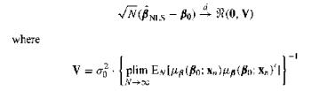
(GNR) Consider the nonlinear conditional regression model $y_u \sim N(\mu(\beta_0; x_n), \sigma^2)$ where ML estimation of $\beta_0$ corresponds to NLS. What is the difference between the Gauss-Newton and the BHHH search directions?
(Identification) Explain why Assumption 14.3(Likelihood Identification. p. 296) does not imply that the information matrix is positive definite, provided that the information matrix exists. (HINT: Is a negative definite Hessian a necessary condition for a local optimum?)
(LMLE) Suggest some explanations for large differences (relative to the estimated sampling variances) between the MLE and some LMLE.
(MLE for Uniform) If the random variable U has the uniform distribution with parameter θ₀, then its p.d.f. is 1(θ₀ ≤ U ≤ θ₀). Given a sample of N realizations {U₁, ..., UN}, the MLE for θ₀ is the largest observed value $\hat{θ}_N$ = U(N).(a) Find the p.d.f. of $\hat{θ}_N$.
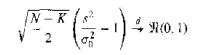
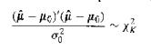
(CLT) Show that the p.d.f. of a chi-square random variable with u degrees of freedom, standardized by its mean and standard deviation, converges to the p.d.f. of the standard normal distribution. Also show how this result relates to the asymptotic distribution of the MLE of the variance in the (μ,
(Information Estimation) Confirm the expression given for the information matrix estimator $ Var[L_n(\theta; \hat{\theta}_N)] $ in Example 15.2. [Hint: Use the normal equations in (14.8) and (14.9) to simplify.]
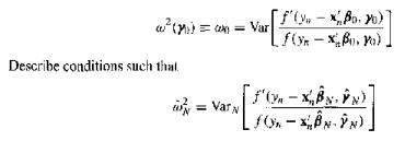
(Symmetric Densities) In such specifications as Example 15.3, we may not know the functional form ofis a consistent estimator of $ \alpha_N^2 $. How would one use this estimator for inference about $ \beta_o $? f'(xBoy) a() == Var f(x-xB) Describe conditions such that =Var fox-BN-N)
Use the results of this chapter to state conditions such that the LAD estimator is a consistent MLE for Example 14.10.
(Normality) The MLF for $ (\mu, \sigma^2) $ in the $ \mathcal{N}(\mu, \sigma^2) $ probability model isShow how the asymptotic distribution of $ \sqrt{N}(\hat{\sigma}^2_N - \sigma^2) $ differs with and without the normality assumption. Suppose that sampling is always i.i.d. and that all the moments
(Dominance) Show that Assumption 14.2(Dominance I) is satisfied by the log-likelihood function for the $ \mathcal{N}(\mu, \sigma^2) $ distribution if the parameter space Θ is bounded and closed, provided that the parameter space bounds $ \sigma^2 $ below by a strictly positive number.
(Unconditional ML) Suppose that the joint p.f. of (U. V) is Fry (u. ;o) fv (; do) for unknown parameter vectors and y). Consider the unconditional alternative to the conditional MLE defined in Definition 28:where fu (o.ao; U) is the marginal p.f. of U. Show that the information matrix of this
(Efficiency of) In this exercise, wo go through some of the steps supporting the relative efficiency of 2 among all unbiased estimators of in the conditional normal model y |X for X full-column rank. (XBIN). (a) Using Jensen's inequality (Lemma D.1), show that if (y, X) is an unbiased estimator of
(Sufficient Statistics) Show that $(\hat{\beta}, s^2)$ are sufficient statistics for $(\beta_0, \sigma^2)$ conditional on $X$, in the conditional normal model $y | X \sim \mathcal{N}(X\beta_0, \sigma^2 I_N)$, for $X$ full-column rank. That is, show that the distribution of $y$ conditional on $X$,
(MLE) Suppose that $U$ is continuously distributed. Suppose also that $N = K$ and that $\hat{\theta}_N = \hat{\theta}(U_1, \dots, U_N)$ is one to one and continuously differentiable. Using the inverse of the MLE as a function of $(U_1, \dots, U_N)$, find an expression for the p.d.f. of the MLE
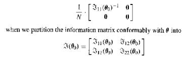
(Restricted ML) Suppose that $\theta_0 = [\theta_{01} \quad \theta_{02}]'$ where $\theta_{02}$ is an $M$-dimensional subvector of $\theta_0 \in R^K$.If $\theta_{02}$ is known, then this knowledge can be imposed in estimation and the Cramér-Rao lower bound reduced. Prove this with the following
[Conditional ML] Show that the Cramér-Rao lower bound for a conditional probability model$f_{W|Z}(w; \theta_2)$ is always greater (in the positive semidefinite sense) than the same bound for the complete joint probability model $f_U(u; \theta_0) = f_{W|Z}(w; \theta_0) f_Z(z; \theta_0)$.
(OLS) In Example 14.11, we showed that the OLS estimator $\hat{\beta}$ is one component of a local maximum of the normal log-likelihood. Prove that this point is a global maximum using the following steps.
(Cramér-Rao) Let $\{U_1, \dots, U_n\}$ be a random sample from the distribution with c.d.f. $F(u; \theta)$, $\theta \in \mathbb{R}^k$. Suppose that $F(u; \theta)$ satisfies conditions that admit the existence of the information matrix. Suppose also that there is an unbiased estimator
(Cramér-Rao) Does Theorem 10 (Cramér-Rao Lower Bound, p. 306) imply that the variance bound can be achieved by a feasible estimator? Explain.
(MLE) Under Assumption 14.1, show that the computation of MLE does not require the specification of the marginal distribution of V when the p.f. of V is invariant to θ₀.
(MLE) Find the MLE for θ₀ in the exponential model:Is the MLE unbiased? Find the information matrix and the variance of the MLE. Is the MLE efficient relative to other unbiased estimators? F(uf) = ifu
(Score Identity) Use the log-likelihood inequality (Lemma 14.1, p. 290) to give an alternative proof of the score identity (Lemma 14.3, p. 300).
is a case in point. For this model,(a) find the score function Lθ(θ) and show that the set of outcomes in which the score is undefined occurs with a probability of zero,(b) find the gradient of the expected value of the log-likelihood function, ∂ E[L(θ)]/∂θ.(c) show that E[Lθ(θ₀)] =
(Score Identity) The score identity (Lemma 14.3, p. 300) still holds if the score function is continuously differentiable except on a set of outcomes that has a probability equal to zero. The Laplace linear regression model described in Examples 14.7, 14.10, and
(Likelihood Identities) Suppose that U is a continuous random variable with the p.d.f. f (u: θ₀), which is twice continuously differentiable in θ₀. Let (U₁, ..., Uₙ) be a random sample of U.(a) Prove that E[Lθ₀(θ₀)] = 0.(h) Suppose also that Var[Lθ(θ₀)] exists. Prove that
Resolve the following paradox: the asymptotic approximation of the distribution of and s implics that we treat as a constant when we draw inferences about Bo but we treat s as a normally distributed random variable when we draw inferences about a
(Almost Sure Convergence) Consider the stochastic sequence $$\{U_n\}$$ whereShow that (U converges in probability to zero but that [UN] does not converge almost surely to zero. Pr(UU): = {} if U=0 N if U-1
(Convergence of Moments) Let $$Z_N \xrightarrow{d} Z$$. Construct an example to show that the limit of $$E[Z_N]$$ may not equal $$E[Z]$$. (HINT: Try constructing a distribution for $$Z_N$$ from the mixture of two distributions with weights that depend on N.)
(Chebychev's LLN) Show that Chebychev's LLN (Theorem 8) need not require independence or identical distributions using the following exceptions to the conditions of the theorem. In each case, use the logic of the theorem's proof to show that $$E_N[U] \xrightarrow{p} E[U]$$ as $$N \to \infty$$.(a)
(Fat Tails) The normal p.l.f. has the thinnest tails of the distributions described in this chupter. (a) Confirm that the ratio of a standard normal p.d.f. over a logistic p.d.f. converges to zero in the tails, as in (13.4). (b) Show that the Laplace and logistic p.d.f.s have tails of comparable
(Mixtures of Normals) Suppose that, conditional on X, each y, is independently and identically distributed as a mixture of normals (Exercise 13.2) with mean x Bo and constant variance. (a) Argue that . y-, and 8 also have conditional p.d.f.s that are also mixtures of normals. (b) Argue that and y-
(Mixture of Normals) A mixture of normal p.d.f.s is one way to generalize the normal distribution.As a simple case, consider the univariate p.d.f.where γ is an additional parameter between 0 and 1.(a) Show that a random variable with this p.d.f. can be generated as a randomized selection of a
(Logistic Distribution) A distribution that is quite similar to the normal is based on the simple c.d.f.called the logistic.(a) Show that F(x) has the properties of a c.d.f.(b) Find the p.d.f. and confirm that it is symmetric about 0.(c) Find the mean and the variance of this distribution.(d) Graph
(Lagrange Multipliers) Show that the numerator of the vector of Lagrange multipliers AR for the restrictions R variance matrix of the Lagrange multipliers. statistic is also a quadratic form in the =r (Exercise 4.15) and the inverse of the
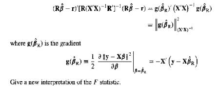
(F Test) Show that the numerator of the statistic in (11.1) can also be expressed a as (RB-r) [R(XX) 'R' (RB-r) = g(BR) (XX)g(BR) where g(B) is the gradient g(BR) = = =-X (y-XBR) 2 Give a new interpretation of the F statistic.
(Ratio of Normals) In the analysis of earnings, we estimated a quadratic function in experience.The ratio of the linear coefficient over twice the quadratic coefficient is the peak of the earnings-experience profile. Find the p.d.f. of the corresponding ratio using the two OLS estimators of these
(RLS Misspecification) Show that all of the elements of the RLS estimator $\hat{\beta}_R$ (Proposition 3, p. 79)may be biased when $R\beta_0 e r$, regardless of whether the elements appear in the restrictions.
Show that the variance ellipse of $\hat{\beta}$ yields the interval estimator with the smallest volume.
(Norm) Let $\Omega$ be a variance matrix. Show that $||v||_\Omega^2 = v'\Omega v$ is a norm on the vector subspace Col($\Omega$).
(Quadratic Forms) Let $\Omega$ be a variance matrix and W a full-column rank matrix such that $WW' = \Omega$.Let $W^+ = (W'W)^{-1}W'$ be the Moore-Penrose generalized inverse of W. Show(a) $P_W = WW^+$ and $W^+y$ is the coefficient vector of W for the orthogonal projection of y onto Col(W),(b) the
(i.i.d.) Show that if the $y_i - x_i'\beta_i$ are i.i.d. conditional on X, then the marginal distribution of $s^2$ is invariant to $\beta_{02}$ and the marginal distribution of the OLS fitted coefficient vector $\hat{\beta}_1$ is invariant to $\beta_{02}$for partitioned regression $X\beta =
(Exact Multicollinearity) Given X, what is the joint conditional distribution of $ \hat{\sigma}^2 $ and $ \hat{\mu} $ if one drops Assumption 3.1(Full Rank, p. 53) from Proposition 10 (Distribution of Variance Estimator, p. 199)?
(Generalized Inverse) Under the conditions of Proposition 9 (Normality of OLS, p. 198), interpretas an application of Lemma 10.7. (-pc) (-) of
(Minimum Chi-Square) Confirm Lemma 10.1(Minimum Chi-Square) for the case in which the subspace S of $ R^N $ is the set of vectors $ \{z_n: n = 1, \dots, N \} \in R^N $ with $ z_n = 0 $ for $ n = 1, \dots, M < N $.
(Confidence Intervals) Using $ \alpha = 0.95$ and values for K and N that you choose, confirm that the critical values $ \chi^2_{K; 1 - \alpha} $ in the infeasible confidence interval (10.7) are smaller than the values $ K F_{K, N - K; 1 - \alpha} $ in the feasible confidence interval (10.10). What
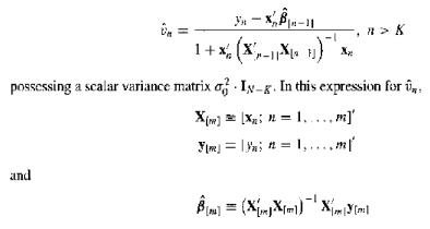
(Recursive Residuals) As in Exercises 8.15 and 9.9, let $ \hat{\beta}_{[m]} $ be the OLS estimator for $ \beta_0 $ using the first $ m $ observations ($ m \ge K $). Under the conditions of Proposition 9 (Normality of OLS, p. 198), show that the $ N - K $ recursive residuals $ y_n - x_n'
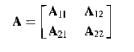
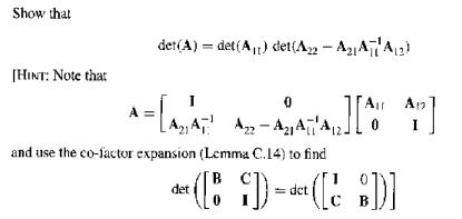
(Partitioned Determinant) Just as there is a useful formula for the inverse of a partitioned matrix, there is a partitioned-matrix determinant formula. Let the square matrix $A$ be partitioned according to All A12 A = LA21 Azz
Let $y \in \mathbb{R}^2$ possess a bivariate normal distribution with mean vector $\mu \in \mathbb{R}^2$ and variance matrix $\Omega = [\omega_{ij}; i, j = 1, 2]$. Find the mean and variance of $y_1$ conditional on $y_2$. Compare this conditional mean with the MMSE linear predictor of $y_1$ given
For the univariate $\mathcal{N}(\mu, \sigma^2)$ distribution, show that(a) the p.d.f. integrates to 1;(b) the mean is finite and equals $\mu$;(c) all odd moments about $\mu$ are 0;(d) the second moment about $\mu$ (the variance) is $\sigma^2$; and(e) the fourth moment about $\mu$ is $3\sigma^4$.
Confirm that the $\mathcal{N}(0, I_N)$ distribution is the product of $N$ univariate standard normal p.d.f.s.
Let $y \sim \mathcal{N}(0, 1)$ and show that $y$ and $y^2$ are uncorrelated but dependently distributed. Find $E[y \mid y^2]$ and $F[y^2 \mid y]$. Using computer software for three-dimensional plotting, graph the joint c.d.f. of $y$ and $y^2$.
(Log-Normal) In addition to functional form and homoskedasticity, the logarithmic transformation of wages makes the marginal distribution of wages more symmetric, and hence closer to normal.(a) Use the 1995 CPS data to confirm this claim(b) Find the log-normal p.d.f. That is, find the p.d.f. of the
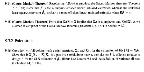
Consider two full-column rank design matrices, X, and X. for the estimation of Ely | X] = XB- Show that if XX-XX is a positive semidefinite matrix, then design B is efficient relative to design A for the OLS estimator of B. IIIINT: Use Lemma 9.1 and the definition of variance ellipses (Definition
(Gauss-Markov Theorem) Prove that XAX = X implies that XA is a projector onto Col(X), as we claimed in our proof of the Gauss Markov theorem (Theorem 7, p. 187) in
(Gauss-Markov Theorem) Resolve the following paradox: the Gauss-Markov theorem (Theorem 7, p. 187) states that is the minimum-variance linear unbiased estimator, whereas the restricted least-squares estimator B is clearly a more efficient linear unbiased estimator when RB = r.
(Full Rank, p. 53), but that the relative efficiency of $$ \hat{\beta}_R $$ to $$ \hat{\beta} $$ does. 9.14 (Gauss-Markov Theorem) Resolve the following paradox: the Gauss-Markov theorem (Theorem 7, p. 187) states that is the minimum-variance linear unbiased estimator, whereas the restricted
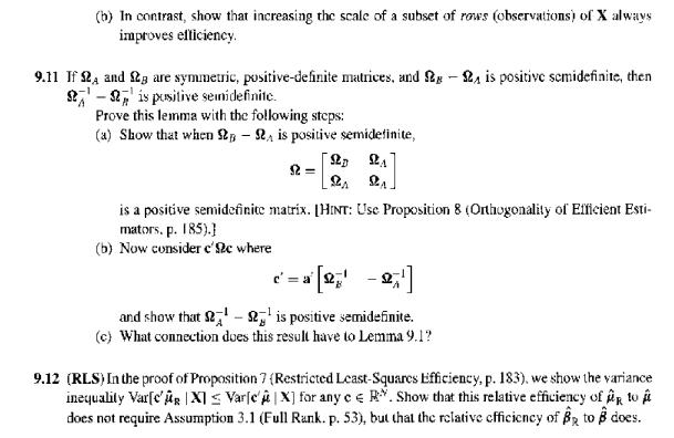
(RLS) In the proof of Proposition 7 (Restricted Least-Squares Efficiency, p. 183), we show the variance inequality $$ Var[c'\hat{\mu}_R | X] \le Var[c'\hat{\mu} | X] $$ for any $$ c \in R^k $$. Show that this relative efficiency of $$ \hat{\mu}_R $$ to $$ \hat{\mu} $$ does not require Assumption
If $$ \Omega_B $$ and $$ \Omega_A $$ are symmetric, positive-definite matrices, and $$ \Omega_B - \Omega_A $$ is positive semidefinite, then$$ \Omega_A^{-1} - \Omega_B^{-1} $$ is positive semidefinite.Prove this lemma with the following steps:(a) Show that when $$ \Omega_B - \Omega_A $$ is positive
Although increasing the scale of X improves the efficiency of the OLS estimator, increasing the scale of a subset of the columns of X does not necessarily improve efficiency. (a) Let X = [X1, X2] and suppose that one may replace X with a X1, where a > 1, before drawing observations on y. Show
Under what circumstances does the distribution of $\hat\beta$ marginal of $X$ hold interest? Describe the marginal variance matrix of $\hat\beta$ under the assumptions of Proposition 5 (Variances of OLS, p. 157). Do the elements of this matrix always exist? If they are finite, how can one estimate
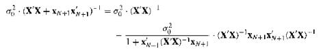
Use Exercise 3.22 to confirm equation (9.1): (XX+X+X+1) = 0 (XX) 1 of 1+x_(XX)-x+ (XX)x+(XX)'
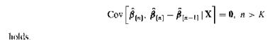
(Partitioned Regression) Let $X_2'X_1 = 0$. We have already seen that such orthogonality implies that algebraically $\hat\beta_1$ is not affected by the presence of $X_2$ in the OLS regression (Example 3.3, Exercise 3.13). Show that in addition $Cov[\hat\beta_1, \hat\beta_2 | X] = 0$, as might be
Let $K = 2$ and $X\beta = X_1 + X_2$. Suppose $X_1'X_2 = X_2'X_1$ and compare $Var[\hat\beta_1 | X]$, $Var[\hat\beta_1 + \hat\beta_2 | X]$, and $Var[\hat\beta_1 - \hat\beta_2 | X]$ as $X_1'X_2 \to X_1'X_1$. Construct a graphic illustration along the lines of Figure 9.5.
Let $E[y \,|\, X] = X_1 \beta_{01} + X_2 \beta_{02}$ and verify $X'X = \sigma_0^2 I$. Draw a geometric representation in two dimensions of an increase in the scale of $X_1$ and $X_2$ leading to a decrease in the sampling variances of $\hat{\beta}$.the coefficients. Show that if $X_1$ and $X_2$ are
(RLS) Show that $Cov[\hat{\beta}_R, \hat{\beta}_R \,|\, X] = Var[\hat{\beta}_R \,|\, X]$ under the assumptions of Proposition 5 (Variances of OLS, p. 157). What does this imply?
(Monte Carlo) Using a computer, generate an artificial data set of 21 observations as follows:(a) Set $w_n = \frac{20}{21}(n-1)$ for $n = 1, \dots, 21$.(b) Set $y_n = w_n^2 + \epsilon_n$ where $\epsilon_n \sim \mathcal{N}(0, \frac{1}{100})$.Using this data set, compute OLS fitted values for each of
Graph the variance ellipse $V_\hat{\beta}$ for the two cases discussed in Example 9.2. Interpret the differences in terms of the effects of increasing multicollinearity on the conditional sampling variance of $\hat{\beta}$. (Hint: Review Figure 8.4.)
(Generalized Inverse) Another generalized inverse of variance matrices follows from the eigenvalue decomposition (Exercise 7.28). Let $ Var[z] = \Omega = RAR^{'} $ be an eigenvalue decomposition of $ \Omega $. Show that a generalized inverse of $ \Omega $ is $ RA^{-} R^{'} $ where $ A^{-} $ is a
(Generalized Inverse) Using the singular-value decomposition (Exercise 7.27) of a positive semi-definite matrix $ \Omega = BHB^{'} $, where H is nonsingular and symmetric and B is full-column rank, construct a generalized inverse for $ \Omega $.
(Image of a Variance Ellipse) Show that the ellipse Va is identically the image of Vy under orthogonal projection on Col(X) using the following steps. (a) Using (8.4) and (8.5), show that VV, and Va =PxV CPXV. (b) Use the fact that y'y y'Pxy for all y to show that PxV, CV.6*8.17 (Generalized
(RLS Variance) Under the assumptions of Proposition 5 (Variances of OLS, p. 157), find the variance matrix of the restricted OLS estimator (Proposition 3, p. 79) in the special case in which we can partition X8=XB+X2B and the restrictions take the form B = 0.
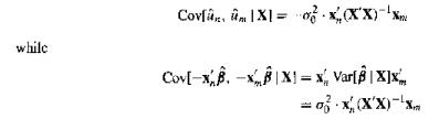
In Proposition 5 the covariance between the fitted residuals yn xB and y-> -xis given (correctly) ashas the opposite sign. Resolve this paradox. while Covf|X|= 0xXX) Cov[-x-xx=x Var[|X]x =0x, (X'X)-xm
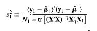
(Subsample Variance) Suppose that you want to estimate the variance σ2 with a subsample of the observations n = 1,..., N1 XB. is an unbiased estimator under the where yyy,' and =l...AN, assumptions of Proposition 6. (HINT: Use the results of Exercise 8.8.) (y)(-) N-tr[(XX) *XX]
(Variance Estimator) The trace of a square matrix A, denoted tr(A), is the sum of its diagonal elements. That is, tr(A) = $$\sum_{j=1}^J a_{jj}$$ where A = [aij; i, j = 1,..., J]. Prove the following properties of matrix traces:(a) If A is a square matrix and c is a scalar, then tr(c·A) =
(Restricted Least Squares) Show that the restricted least-squares program (4.2) is equivalent tosubject to $$Kβ = r$$when rank(X) = K and Assumption 7.1(Second Moments, p. 130) holds. min(-8) Var[|X]' (B-B) subject to K=r B
(Forecast Variance) Suppose that you have sample data on a pair of variables: ((xn, yn); n = 1,..., N). Under the assumptions of Proposition 5 (Variances of OLS, p. 157), find the conditional variance of the forecast error of the OLS forecast $$β_1 + β_2x_{N+1}$$ for yN+1 given {xn; n = 1,...,
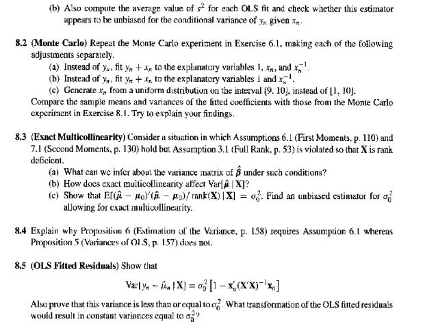
(OLS Fitted Residuals) Show thatAlso prove that this variance is less than or equal to $\sigma^2$. What transformation of the OLS fitted residuals would result in constant variances equal to $\sigma^2$? Varly-X]=[1-xx(XX)x]
Explain why Proposition 6 (Estimation of the Variance, p. 158) requires Assumption 6.1 whereas Proposition 5 (Variances of OLS, p. 157) does not.
(Exact Multicollinearity) Consider a situation in which Assumptions 6.1(First Moments, p. 110) and 7.1(Second Moments, p. 130) hold but Assumption 3.1(Full Rank, p. 53) is violated so that X is rank deficient.(a) What can we infer about the variance matrix of $\hat{\beta}$ under such conditions?(b)
(Monte Carlo) Repeat the Monte Carlo experiment in Exercise 6.1, making each of the following adjustments separately.(a) Instead of $y_i$, fit $y_i + x_i$ to the explanatory variables 1, $x_i$, and $x_i^{-1}$.(b) Instead of $y_i$, fit $y_i + x_i x_i$ to the explanatory variables 1 and
(Monte Carlo) Repeat the Monte Carlo experiment in Exercise 6.1 with the following changes. (a) In addition to sample means, compute the sample variances and covariances of the three OLS fitted coefficients. Compare these values with their population counterparts.(b) Also compute the average value
Show that one can always view the generalized Euclidean inner product $$x'\Omega y$$ of two vectors x and y with a nonsingular variance matrix $$\Omega$$ as the ordinary Euclidean inner product of a linear transformation of the vectors.
(Eigenvalue Decomposition) In econometrics, another popular decomposition for symmetric matrices is the eigenvalue decomposition. It is always possible to find an orthogonal matrix R and a diagonal matrix A such that $$\Omega = RAR'$$. The columns of R are called eigenvectors and the diagonal
(Singular Value Decomposition) Let A be a real symmetric matrix. Let B be a full-column rank matrix such that Col(B) = Col(A) so that the columns of B are a basis for the columns of A.(a) Given A, how could you find such a B?(b) Show that $$A = BC$$ where C has the same dimensions as B.(c) Show
Show that the only positive-definite orthogonal projection matrix is the identity matrix.
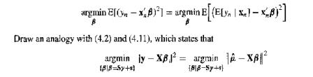
(Restricted Least Squares) Given that the second moments of yₙ and xᵢ exist, show that argmin [ -x)] = argmin E[(E[y | x1 = x)] Draw an analogy with (4.2) and (4.11), which states that argmin ly XBargmin -X|| (B|B=Sy+s] 818-Sy-s
Under Assumptions 6.1(First Moments, p. 110) and 7.1(Second Moments, p. 130), find Var[μ̂ | X](a) when X is full-column rank and(b) when X is rank deficient (not full-column rank).
Showing 100 - 200
of 618
1
2
3
4
5
6
7
Step by Step Answers