New Semester
Started
Get
50% OFF
Study Help!
--h --m --s
Claim Now
Question Answers
Textbooks
Find textbooks, questions and answers
Oops, something went wrong!
Change your search query and then try again
S
Books
FREE
Study Help
Expert Questions
Accounting
General Management
Mathematics
Finance
Organizational Behaviour
Law
Physics
Operating System
Management Leadership
Sociology
Programming
Marketing
Database
Computer Network
Economics
Textbooks Solutions
Accounting
Managerial Accounting
Management Leadership
Cost Accounting
Statistics
Business Law
Corporate Finance
Finance
Economics
Auditing
Tutors
Online Tutors
Find a Tutor
Hire a Tutor
Become a Tutor
AI Tutor
AI Study Planner
NEW
Sell Books
Search
Search
Sign In
Register
study help
business
essential statistics
Essential Statistics 1st Edition David S Moore - Solutions
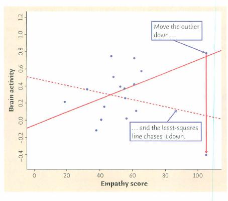
5.32 Our brains don't like losses. Exercise 4.24 (page 86)describes an experiment that showed a linear relationship be tween how sensitive people are to monetary losses ("behavioral loss aversion") and activity in one patt of their brains ("neural loss aversion").(a) Make a scatterplot with neural
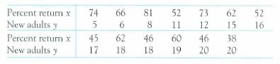
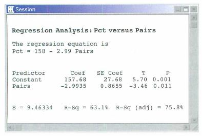
5.31 Sparrowhawk colonies. One of nature's patterns con nects the percent of adult bitds in a colony that return from the ptevious year and the number of new adults that join the colony. Here are data for 13 colonies of sparrowhawks:'^You saw in Exercise 4.23 that there is a moderately strong
5.30 Sisters and brothers. How strongly do physical charac teristics of sisters and brothers correlate? Here are data on the heights (in inches) of 11 adult pairs:'^Brother i 71 68 66 67 70 71 70 73 72 65 66 Sister ! 69 64 65 63 65 62 65 64 66 59 62(a) Use your calculator or software to find the
5.29 Going to class. A study of class attendance and grades among first-year students at a state university showed that in general students who attended a higher percent of their classes earned higher grades. Class attendance explained 16% of the variation in grade index among the students. What is
5.28 What's my grade? In Professor Friedman's economics course the correlation between the students' total scores prior to the final examination and their final examination scores is r = 0.6. The pre-exam totals for all students in the course have mean 280 and standard deviation 30. The final-exam
5.27 Husbands and wives. The mean height of American women in their twenties is about 64 inches, and the standard deviation is about 2.7 inches. The mean height of men the same age is about 69.3 inches, with standard deviation about 2.8 inches. Suppose that the correlation between the heights of
5.26 Merlins breeding. Exercise 4.36 (page 89) gives data on the number of breeding pairs of merlins in an isolated area in each of nine years and the percent of males who returned the next year. The data show that the percent returning is lower after successful breeding seasons and that the
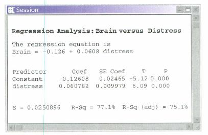
5.25 Does social rejection hurt? Exercise 4-37 (page 89)gives data from a study that shows that social exclusion causes"real pain." That is, activity in an area of the brain that re sponds to physical pain goes up as distress from social exclusion goes up. A scatterplot shows a moderately strong
5.24 Measuring water quality. Biochemical oxygen demand(BOD) measures organic pollutants in water by measuring the amount of oxygen consumed by microorganisms that break down these compounds. BOD is hard to measure accurately.Total organic carbon (TOO) is easy to measure, so it is common to measure
5.23 Penguins diving. A study of king penguins looked for a relationship between how deep the penguins dive to seek food and how lotig they stay underwater. There is a linear rela tionship that is different for different penguins. The study re port gives a scatterplot for one penguin titled "The
5.22 Because elderly people may have difficulty standirig to have their heights measured, a study looked at predicting over all height from height to the knee. Here are data (in centimetets)for five elderly men:Knee height x Height y 57.7 192.1 47.4 153.3 43.5 146.4 44.8 162.7 55.2 169.1 Use your
5.21 In addition to the regression line in Exercise 5.18, the report on the Mumbai measurements says that = 0.95. This suggests that(a) although armspan and height are correlated, armspan does not predict height very accurately.(b) height increases by ^0.95 = 0.97 cm for each additional centimeter
5.20 By looking at the equation of the least-squares regression line in Exercise 5.18, you can see that the correlation between height and armspan is(a) greater than zero.(b) less tharr zero.(c) Can't tell without seeing the data.
5.19 According to the regression line in Exercise 5.18, the pre dicted height of a child with armspan 100 cm is about(a) 106.4 cm. (b) 99.4 cm. (c) 93 cm.
5.18 Measurements on young children in Mumbai, India, found this least-squares line for predicting height y from armspan x:'y = 6.4 4- 0.93x Measurements are in centimeters (cm). How much on the av erage does height increase for each additional centimeter of armspan?(a) 0.93 cm. (b) 6.4 cm. (c)
5.17 Smokers don't live as long (on the average) as nonsmokers, and heavy smokers don't live as long as light smokers. You regress the age at death of a group of male smokers on the num ber of packs per day they smoked. The slope of your regression line(a) will be greater than 0.(b) will be less
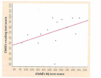
5.16 The slope of the line in Figure 5.7 is closest to(a)-l. (b)0. (c) 1.
5.15 Figure 5.7 is a scatterplot of reading test scores against IQ test scores for 14 fifth-grade children. The line is the leastsquares regression line for predicting reading score from IQ score. If another child in this class has IQ score 110, you pre dict the reading score to be close to(a) 50.
5.14 To earn more, get married? Data show that men who are married, and also divorced or widowed men, earn quite a bit more than men the same age who have never been married. This does not mean that a man can raise his income by getting married, be cause men who have never been married are
5.13 Education and income. There is a strong positive association between workers' educa tion and their income. For example, the Census Bureau reports that the ijuedian income of young adults (ages 25 to 34) who work full-time increases from $20,641 for those with less than a ninth-grade education
5.12 Another reason not to smoke? A stop-smoking booklet says, "Children of mothers who smoked during pregnancy scored nine points lower on intelligence tests at ages three and four than childreia of nonsmokers." Suggest some lurking variables that may help explain the association between smoking
5.11 Is math the key to success in college? A College Board study of 15,941 high school graduates found a strong correlation between how much math minority students took in high school and their later success in college. News articles quoted the head of the College Board as saying that "math is the
5.10 The endangered manatee. Table 41 (page 77) gives 31 years' data on boats registered in Florida and manatees killed by boats. Figure 4.2 (page 78) shows a strong positive linear relationship. The correlation is r = 0.947.(a) Find the equation of the least-squares line for predicting manatees
5.9 Outsourcing by airlines. Exercise 4.4 (page 76) gives data for 14 airlines on the percent of rnajor maintenance outsourced and the percent of flight delays blamed pn the airline.(a) Make a scatterplot with outsourcing percent as x and delay percent as y. Hawaiian Airlines is a high outlier in
5.8 Do heavier people burn more energy? Return to the data of Exercise 5.4 (page 95)on lean body mass and metabolic rate. We will use these data to illustrate influence.(a) Make a scatterplot of the data that is suitable for predicting metabolic rate from body mass, with two new points added. Point
5.7 Residuals by hand. In Exercise 5.3 you found the equation of the least-squares line for predicting the number of days y until gorillas in a social group begin to die in an Ebola virus epidemic from the "distance" x from the first group infected.(a) Use the equation to obtain the 6 residuals
5.6 Growing corn. Exercise 4.27 (page 85) gives data from an agricultural experiment. The purpose of the study was to see how the yield of corn changes as we change the planting rate (plants per acre).(a) Make a scatterplot of the data. (Use a scale of yields from 100 to 200 bushels per acre.)Find
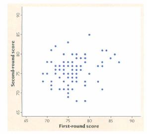
5.5 How useful is regression? Figure 4.6 (page 85) displays the relationship between golfers' scores on the first and second rounds of the 2007 Masters Tournament. The cor relation isr = 0.192. Exercise 4.25 gives data on solar radiation dose (SRD) and concen tration of dimethyl sulflde (DMS) over
5.4 Do heavier people burn more energy? We have data on the lean body mass and resting metabolic rate for 12 women who are subjects in a study of dieting. Lean body mass, given in kilograms, is a person's weight leaving out all fat. Metabolic rate, in calories burned per 24 hours, is the rate at
5.3 Ebola and gorillas. In Exercise 4.8 (page 80), you looked at the spread of an outbreak of the deadly Ebola virus among gorillas in the Congo. The data give a measure of the distance of each group of gorillas from the first group infected and the number of days until deaths began in each later
5.2 What's the line? You use the same bar of soap to shower each morning. The bar weighs 80 grams when it is new. Its weight goes down by 6 grams per day on the average. What is the equation of the regression line for predicting weight from days of use?
5.1 City mileage, highway mileage. We expect a car's highway gas mileage to he related to its city gas mileage. Data for all 1198 vehicles in the government's 2008 Fuel Economy Guide give the regression line highway mpg = 4.62 4- (1.109 x city mpg) for predicting highway mileage from city
4.37 Does social rejection hurt? We often describe our emotional reaction to social rejection as "pain." Does social rejection cause activity in areas of the brain that are known to be activated by physical pain? If it does, we really do experience social and physical pain in similar ways. Psycholo
4.36 Merlins breeding. The percent of an animal species in Ibithe wild that survive to breed again is often lower following a successful breeding season. A study of merlins (small falcons)in northern Sweden observed the number of breeding pairs in an isolated area and the percent of males (banded
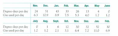
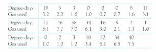
4.35 Saving energy with solar panels. We have data w from a house in the Midwest that uses natural gas for heat ing. Will installing solar panels reduce the amount of gas con sumed? Gas consumption is higher in cold weather, so the rela tionship between outside temperature and gas consumption is
4.34 Brighter sunlight? The brightness of sunlight at the earth's surface changes over time depending on whether the earth's atmosphere is more or less clear. Sun light dimmed between 1960 and 1990. After 1990, air pollu tion dropped in industrial countries. Did sunlight brighten?Here are data from
4.33 Sloppy writing about correlation. Each of the follow ing statements contains a blunder. Explain in each case what is wrong.(a) "There is a high correlation between the gender of Amer ican workers and their income."(b) "We found a high correlation (r = 1.09) between stu dents' ratings of
4.32 Teaching and research. A college news paper interviews a psychologist about student ratings of the teaching of faculty members. The psychologist says, "The evidence indicates that the correlation between the research productiv ity and teaching rating of faculty members is close to zero."The
4.31 Statistics for investing. A mutual funds company's newsletter says, "A well-diversified portfolio includes assets with low correlations." The newsletter includes a table of cor relations between the returns on various classes of investments.For example, the correlation between municipal bonds
4.30 The effect of changing units. Changing the units of measurement can dramatically alter the appearance of a scatterplot.Return to the data on knee height and overall height in Exercise 4-18:Knee height x Height y 57.7 192.1 47.4 153.3 43.5 146.4 44.8 162.7 55.2 169.1 Both heights are measured
4.29 Thinking about correlation. Exercise 4-21 presents data on the heights of women and of the men they date.(a) If heights were measured irr centimeters rather than inches, how would the correlation change? (There are 2.54 centimeters in an inch.)(b) How would r change if all the men were 6
4.28 Attracting beetles. To detect the presence of harmful insects in farm fields, we can put up boards covered with a sticky material and examine the insects trapped on the boards. Which colors attract insects best? Experimenters placed six boards of each of four colors at random locations in a
4.27 How many corn plants are too many? How much corn per acre should a farmer plant to obtain the highest yield?Too few plants will give a low yield. On the other hand, if there are too many plants, they will compete with each other and yields will fall. To find the best planting rate, plant at
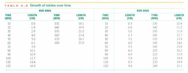
4.26 How fast do icicles grow? Japanese researchers mea sured the growth of icicles in a cold chamber under various conditions of temperature, wind, and water flow.'^ Table 4.2 contains data produced under two sets of conditions. In both cases, there was no wind and the temperature was set at —
4.25 Sulfur, the ocean, and the sun. Sulfur in the atmo sphere affects climate by influencing formation of clouds. The main natural source of sulfur is dimethyl sulfide (DMS) pro duced by small organisms in the upper layers of the oceans.DMS production is in turn influenced by the amount of en ergy
4.24 Our brains don't like losses. Most people dislike losses more than they like gains. In money terms, people are about as sensitive to a loss of $10 as to a gain of $20. To discover what parts of the brain are active in decisions about gain and loss, psychologists presented subjects with a
4.23 Sparrowhawk colonies. One of nature's patterns con nects the percent of adult birds in a colony that return from the previous year and the number of new adults that join the colony. Here are data for 13 colonies of sparrowhawksf^Percent return : 74 66 81 52 73 62 52 45 62 46 60 46 38 New
4.22 Coffee and deforestation. Coffee is a leading export from several developing countries. When coffee prices are high, farmers often clear forest to plant more coffee trees. Here are five years of data on prices paid to coffee growers in In donesia and the percent of forest area lost in a
4.21 Data on dating. A student wonders if tall women tend to date taller men than do short women. She measures herself, her dormitory roommate, and the women in the adjoining rooms;then she measutes the next man each woman dates. Idere are the data (heights in inches):Women (x) i 66 Men(y) I 72 64
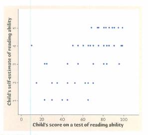
4.20 Can children estimate their own reading ability? To study this question, investigators asked 60 fifth-grade children to estimate their own reading ability, on a scale from 1 (low) to 5 (high). Figure 4.7 is a scatterplot of the children's estimates(response) against their scores on a reading
4.19 Scores at the Masters. The Masters is one of the four major golf tournaments. Figure 4.6 is a scatterplot of the scores for the first two rounds of the 2007 Masters for all of the golfers entered. Only the 60 golfers with the lowest two-round total advance to the final two rounds. The plot has
4.18 Because elderly people may have difficulty standing to have their heights measured, a study looked at predicting over all height from height to the knee. Following are data (in cen timeters) for five elderly men.Use your calculator or software: the correlation between knee height and overall
4.17 For a biology project, you measure the weight in grams and the tail length in millimeters of a group of mice. Thecorrelation is r = 0.7. If you had measured tail length in cen timeters instead of millimeters, what would be the correlation?(There are 10 millimeters in a centimeter.)(a) 0.7/10 =
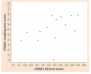
4.16 The points on a scatterplot lie very close to the line whose equation is 31 = 4 — 3x. The correlation between x and y is close to(a) -3. (b) -1. (c) 1.
4.15 If the correlation between two variables is close to 0, you can conclude that a scatterplot would show(a) a strong straight-line pattern.(b) a cloud of points with no visible pattern.(c) no straight-line pattern, but there might be a strong pat tern of another form.
4.14 If we leave out the low outlier, the correlation for the re maining 13 points in Figure 4.5 is closest to(a) 0.5. (b) -0.5. (c) 0.95.
4.13 Figure 4.5 is a scatterplot of reading test scores against IQ test scores for 14 fifth-grade children. There is one low outlier in the plot. The IQ and reading scores for this child are(a) IQ = 10, reading = 124.(b) IQ = 124, reading = 72.(c) IQ =: 124, reading = 10.
4.11 Strong asscciation but no correlation. The gas mileage of an automobile first in creases and then decreases as the speed increases. Suppose that this relationship is very regular, as shown by the following data on speed (miles per hour) and mileage (miles per gallon):Speed : 20 30 40 50 60
4.10 Changing the correlation. Use your calculator or software to demonstrate how outliers can affect correlation.(a) What is the correlation between lean body mass and metabolic fate for the 12 women in Exercise 4.3?(b) Make a scatterplot of the data with two new points added. Point A: mass 65
4.9 Changing the units. The healing rates plotted in Figure 4.4(c) are measured in mi crometers (millionths of a meter) per hour. The correlation between healing rates for the two front limbs of newts is r = 0.358. If the measurements were made in inches per day, would the correlation change?
4.8 Ebola and gorillas. An outbreak of the deadly Ebola virus in 2002 and 2003 killed 91 of the 95 gorillas in 7 home ranges in the Congo. To study the spread of the virus, measure"distance" by the number of home ranges separating a group of gorillas from the first group infected. Here are data on
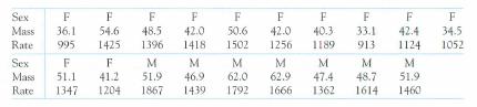
4.7 Do heavier people burn more energy? The study of dieting described in Exercise 4-3 collected data on the lean body mass (in kilograms) and metabolic rate (in calories) for both female and male subjects:(a) Make a scatterplot of metabolic rate versus lean body mass for all 19 subjects. Use
4.6 Outsourcing by airlines. Does your plot for Exercise 4.4 show a positive association between maintenance outsourcing and delays caused by the airline? One airline is a high outlier in delay percent. Which airline is this? Aside from the outlier, does the plot show a roughly linear form? Is the
4.5 Do heavier people burn more energy? Describe the direction, form, and strength of the relationship between lean body mass and metabolic rate, as displayed in your plot for Exercise 4.3.
4.4 Outsourcing by airlines. Airlines have increasingly outsourced the maintenance of their planes to other companies. Critics say that the maintenance may be less carefully done, so that outsourcing creates a safety hazard. As evidence, they point to government data on percent of major maintenance
4.2 Coral reefs. How sensitive to changes in water temperature are coral reefs? To find out, measure the growth of corals in aquariums where the water temperature is controlled at different levels. Growth is measured by weighing the coral before and after the experi ment. What are the explanatory
4.1 Explanatory and response variables? You have data on a large group of college stu dents. Here are four pairs of variables measured on these students. For each pair, is it more reasonable to simply explore the relationship between the two variables or to view one of the variables as an
3.46 Are the data Normal? Soil penetrability. Table 2.5(page 48) gives data on the penetrability of soil at each of three levels of compression. We might expect the penetrability of specimens of the same soil at the same level of compression to follow a Normal distribution. Make stemplots of the
3.45 Are the data Normal? Monsoon rains. Here are the amounts of summer monsoon rainfall (millimeters) for India in the 100 years 1901 to 2000:"722.4 736.8 866.2 877.6 728.7 739.2 1020.5 887.0 852.4 784.7 792.2 806.4 869.4 803.8 958.1 793.3 810.0 653.1 735.6 785.0 861.3 784.8 823.5 976.2 868.6
3.44 Are the data Normal? Fruit fly thorax lengths. Here are the lengths in millimeters of the thorax for 49 male fruit flies:"0.64 0.64 0.64 0.68 0.68 0.68 0.72 0.72 0.72 0,72 0.74 0.76 0.76 0.76 0.76 0.76 0.76 0.76 0.76 0.78 0.80 0.80 0.80 0.80 0.80 0.82 0.82 0.84 0.84 0.84 0.84 0.84 0.84 0.84
3.43 Are the data Normal? Acidity of rainfall. Exercise 3.27 concerns the acidity (measured by pH) of rainfall. A sample of 105 rainwater specimens had mean pH 5.43, standard de viation 0.54, and five-number summary 4.33, 5.05, 5.44, 5.79, 6.81.'°(a) Compare the mean and median and also the
3.42 Normal is only approximate: ACT scores. Scores on the ACT test for the 2007 high school graduating class had mean 21.2 and standard deviation 5.0. In all, 1,300,599 students in this class took the test. Of these, 149,164 had scores higher than 27 and another 50,310 had scores ex actly 27. ACT
3.41 Normal is only approximate: IQ test scores. The fol lowing lists give the IQ test scores of 31 seventh-grade girls in a Midwest school district.^114 100 104 89 102 91 114 114 103 105 108 130 120 132 111 128 118 119 86 72 111 103 74 112 107 103 98 96 112 112 93(a) We expect IQ scores to be
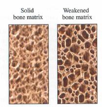
3.40 Osteoporosis. Osteoporosis is a condition in which the bones become brittle due to loss of minerals. To diagnose osteo porosis, measure bone mineral density (BMD). BMD is usually reported in standardized form. The standardization is based on a population of healthy young adults. The World
3.39 Grading managers. Some companies "grade on a bell curve" to compare the performance of their managers and professional workers. This forces the use of some low perfor mance ratings so that not all workers are listed as "above aver age." Ford Motor Company's "performance management pro cess"
3.38 Heights of men and women. The heights of women aged 20 to 29 follow approximately the N(64, 2.7) distribution.Men the same age have heights distributed as N(69.3, 2.8).What percent of young men are shorter than the mean height of young women?
3.37 Heights of men and women. The heights of women aged 20 to 29 follow approximately the N(64, 2.7) distribution.Meri the same age have heights distributed as N(69.3, 2.8).What percent of young women are taller than the mean height of young men?
3.36 Perfect SAT scores. It is possible to score higher than 1600 on the SAT, but scores 1600 and above are reported as 1600. In 2007 the distribution of SAT scores (combining math ematics and reading) was close to Normal with mean 1021 and standard deviation 211.® What proportion of 2007 SAT
3.35 What's your percentlle? Reports on a student's ACT or SAT usually give the percentile as well as the actual score.The percentile is just the cumulative proportion stated as a per cent: the percent of all scores that were lower than this one. In 2007, composite ACT scores were close to Normal
3.34 Quintlles. The quintiles of any distribution are the val ues with cumulative proportions 0.20, 0.40, 0.60, and 0.80.What are the quintiles of the distribution of gas mileage?
3.33 The middle half. The quartiles of any distribution are the values with cumulative proportions 0.25 and 0.75. They span the middle half of the distribution. What are the quartiles of the distribution of gas mileage?
3.32 The top 10%. How high must a 2008 vehicle's gas mileage be in order to fall in the top 10% of all vehicles?(The distribution omits a few high outliers, mainly hybrid gaselectric vehicles.)
3.31 In my Chevrolet. The 2008 Chevrolet Malihu with a four-cylinder engine has combined gas mileage 25 mpg. What percent of all vehicles have worse gas mileage thaia the Malibu?
3.30 Making tablets. A pharmaceutical mariufacturer forms tablets by compressing a granular material that contains the ac tive ingredient and various fillers. The force in kilograms (kg)applied to the tablets varies a bit, with the N(11.5, 0.2) dis tribution. The process specifications call for
3.29 A milling machine. Automated manufacturing opera tions are quite precise but still vary, often with distributions that are close to Normal. The width in inches of slots cut by a milling machine follows approximately the N(0.8750, 0.0012)disttihution. The specifications allow slot widths
3.28 Runners. In a study of exercise, a large group of male runners walk on a treadmill for 6 minutes. Their heart rates in beats per minute at the end vary from runner to runner ac cording to the N(104, 12.5) distribution. The heart rates for male nonrunners after the same exercise have the N(
3.27 Acid rain? Emissions of sulfur dioxide by industry set off chemical changes in the atmosphere that result in "acid rain."The acidity of liquids is measured by pH on a scale of 0 to 14.Distilled water has pH 7.0, and lower pH values indicate acid ity. Normal rain is somewhat acidic, so acid
3.25 Standard Normal drill.(a) Find the number z such that the proportion of observa tions that are less than ?: in a standard Normal distribution is 0.8.(b) Find the number ? such that 35% of all observations from a standard Normal distribution are greater than z-3.26 Running a mile. After the
3.24 Standard Normal drill. Use Table A to find the pro portion of observations from a standard Normal distribution that falls in each of the following regions. In each case, sketch a standard Normal curve and shade the area representing the region.(a) ? < -2.25 (b) ? > -2.25 (c) ? > 1.77(d) -2.25
3.23 Low IQ test scores. Scores on the Wechsler Adult In telligence Scale (WAIS) are approximately Normal with mean 100 and standard deviation 15. People with WAIS scores be low 70 are considered mentally retarded when, for example, ap plying for Social Security disability benefits. According to
3.22 Daily activity. It appears that people who are mildly obese are less active than leaner people. One study looked at the average number of minutes per day that people spend stand ing or walking.^ Among mildly obese people, minutes of activ ity varied according to the N(373, 67) distribution.
3.21 The scores of adults on an IQ test are approximately Nor mal with mean 100 and standard deviation 15. Corinne scores 118 on such a test. She scores higher than what percent of all adults?(a) About 12% (b) About 88% (c) About 98%
3.20 The scores of adults on an IQ test are approximately Nor mal with mean 100 and standard deviation 15. Corinne scores 118 on such a test. Her ?:-score is about(a) 1.2. (b) 7->87. (c) 18.
3.19 The scores of adults on an IQ test are approximately Nor mal with mean 100 and standard deviation 15. The organiza tion MENSA, which calls itself "the high IQ society," requires an IQ score of 130 or higher for membership. What percent of adults would qualify for membership?(a) 95% (b) 5% (c)
3.18 The length of human pregnancies from conception to birth varies according to a distribution that is approximately Normal with mean 266 days and standard deviation 16 days.95% of all pregnancies last between(a) 250 and 282 days. (b) 234 and 298 days,(c) 218 and 314 days.
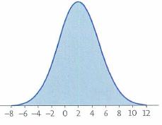
3.17 The standard deviation of the Normal distribution in Fig ure 3.12 is(a) 2. (b)3. (c)5.
3.16 Figure 3.12 shows a Normal curve. The mean of this dis tribution is(a) 0. (b) 2. (c) 3. -8-6-4-2 0 2 4 6 8 10 12
3.15 Which of these variables is least likely to have a Normal distribution?(a) Income per person for 150 different countries(b) Lengths of 50 newly hatched pythons(c) Heights of 100 white pine trees in a forest
3.14 Fruit files. The thorax lengths in a population of male fruit flies follow a Norrnal distri bution with mean 0.800 millimeters (mm) and standard deviation 0.078 mm. What are the median and the first and third quartiles of thorax length?
3.13 Table A. Use Table A to find the value ? of a standard Normal variable that satisfies each of the following conditions. (Use the value of ? from Table A that comes closest to satisfyirig the condition.) In each case, sketch a standard Normal curve with your value of z marked on the axis.(a)
Showing 800 - 900
of 2398
First
2
3
4
5
6
7
8
9
10
11
12
13
14
15
16
Last
Step by Step Answers