New Semester Started Get 50% OFF Study Help! --h --m --s Claim Now

Question Answers

Textbooks

Find textbooks, questions and answers

Oops, something went wrong!

Change your search query and then try again

Result Not Found

Books FREE
Study Help
Tutors
AI Study Planner NEW
Sell Books

Search
Sign In
Register

study help
business
probability statistics

The Basic Practice Of Statistics 8th Edition David S. Moore, William I. Notz, Michael A. Fligner - Solutions

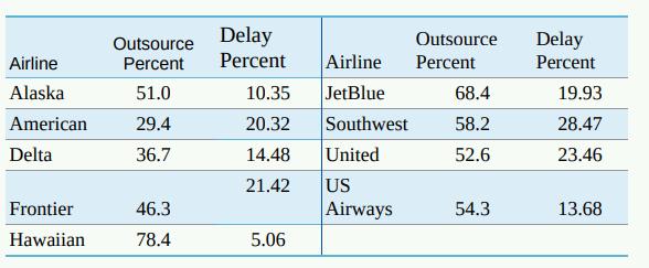
4.5 Outsourcing by Airlines. Airlines have increasingly outsourced the maintenance of their planes to other companies. A concern voiced by critics is that the maintenance may be less carefully done so that outsourcing creates a safety hazard. In addition, flight delays are often due to maintenance
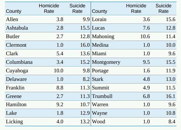
4.4 Death by Intent. Homicide and suicide are both intentional means of ending a life. However, the reason for committing a homicide is different from that for suicide, and we might expect homicide and suicide rates to be uncorrelated. On the other hand, both can involve some degree of violence, so
4.3 Predicting Life Expectancy. Identifying variables that can be used to predict life expectancy is important for insurance companies, economists, and policymakers. Several researchers have investigated the extent to which poverty level can be used to predict life expectancy. Name two other
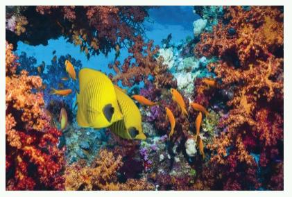
4.2 Coral Reefs. How sensitive to changes in water temperature are coral reefs? To find out, scientists examined data on sea surface temperatures and coral growth per year at locations in the Gulf of Mexico and the Caribbean Sea. What are the explanatory and response variables? Are they categorical
4.1 Explanatory and Response Variables? You have data on a large group of college students. Here are four pairs of variables measured on these students. For each pair, is it more reasonable to simply explore the relationship between the two variables or to view one of the variables as an
3.54 Grading managers. In Exercise 3.44, we saw that Ford Motor Company once graded its managers in such a way that the top 10% received an A grade, the bottom 10% a C, and the middle 80% a B. Let's suppose that performance scores follow a Normal distribution. How many standard deviations above and
3.53 APPLET Where are the quartiles? How many standard deviations above and below the mean do the quartiles of any Normal distribution lie? (Use the standard Normal distribution to answer this question.)
3.52 How accurate is 68-95-99.7? The 68-95-99.7 rule for Normal distributions is a useful approximation. To see how accurate the rule is, drag one flag across the other so that the applet shows the area under the curve between the two flags.(a) Place the flags 1 standard deviation on either side of
3.51 Are the data Normal? Weight of females in their 20s. Many body measurements of people of the same sex and similar ages such as height and upper arm length follow a Normal distribution reasonably closely. Weights, on the other hand, are not Normally distributed. The NHANES survey of 2009-
3.50 Are the data Normal? Monsoon rains. Here are the amounts of summer monsoon rainfall (millimeters) for India in the 100 years 1901 to 2000:16 MONSOON 722.4 792.2 861.3 750.6 716.8 885.5 777.9 897.5 889.6 935.4 736.8 806.4 784.8 898.5 781.0 951.1 1004.7 651.2 885.0 719.4 866.2 869.4 823.5 863.0
3.49 Are the data normal? SAT mathematics scores. Georgia Southern University 3.49 (GSU) had 2786 students with regular admission in its freshman class of 2015. For each student, data are available on his/her SAT and ACT scores, if taken; high school GPA; and the college within the university to
3.48 Are the data Normal? Acidity of rainfall. Exercise 3.31 (page 95) concerns the acidity (measured by pH) of rainfall. A sample of 105 rainwater specimens had mean pH 5.43; standard deviation 0.54; and five-number summary 4.33, 5.05, 5.44, 5.79, 6.81.14 (a) Compare the mean and median and also
3.47 Are the data Normal? Returns on stocks. The return on a stock is the change in its market price plus any dividend payments made. Total return is usually expressed as a percent of the beginning price. Exercise 1.32 provides a histogram of the distribution of the monthly returns for all stocks
3.46 Normal is only approximate: ACT scores. Composite scores on the ACT test for the 2015 high school graduating class had mean 21.0 and standard deviation 5.5. In all, 1,924,436 students in this class took the test. Of these, 205,584 had scores higher than 28, and another 60,551 had scores
3.45 Osteoporosis. Osteoporosis is a condition in which the bones become brittle due to loss of minerals. To diagnose osteoporosis, an elaborate apparatus measures bone mineral density (BMD). BMD is usually reported in standardized form. The standardization is based on a population of healthy young
3.44 Grading managers. Some companies "grade on a bell curve" to compare the performance of their managers and professional workers. This forces the use of some low performance ratings so that not all workers are listed as "above average." Ford Motor Company's "performance management process" for
3.43 A surprising calculation. Changing the mean and standard deviation of a Normal distribution by a moderate amount can greatly change the percent of observations in the tails. Suppose a college is looking for applicants with SAT math scores 750 and above.(a) In 2015, the scores of men on the
3.42 Weights aren't normal. The heights of people of the same sex and similar ages follow a Normal distribution reasonably closely. Weights, on the other hand, are not Normally distributed. The weights of women aged 20-29 in the United States have mean 161.9 pounds and median 149.4 pounds. The
3.41 Heights of men and women. The heights of women aged 20-29 follow approximately the N(64.2, 2.8) distribution. Men the same age have heights distributed as N(69.4, 3.0). What percent of men aged 20-29 are taller than the mean height of women aged 20-29?
3.40 Perfect SAT scores. It is possible to score higher than 1600 on the combined mathematics and reading portions of the SAT, but scores 1600 and above are reported as 1600. The distribution of SAT scores (combining mathematics and reading) in 2014 was close to Normal with mean 1010 and standard
3.39 What's your percentile? Reports on a student's test score such as the SAT or a child's height or weight usually give the percentile as well as the actual value of the variable. The percentile is just the cumulative proportion stated as a percent: the percent of all values of the variable that
3.38 Quintiles. The quintiles of any distribution are the values with cumulative proportions 0.20, 0.40, 0.60, and 0.80. What are the quintiles of the distribution of gas mileage?
3.37 The middle half. The quartiles of any distribution are the values with cumulative proportions 0.25 and 0.75. They span the middle half of the distribution. What are the quartiles of the distribution of gas mileage?
3.36 The top 15%. How high must a 2016 vehicle's gas mileage be to fall in the top 15% of all vehicles?
3.35 I love my bug! The 2016 Volkswagen Beetle with a four-cylinder 1.8-L engine and automatic transmission has combined gas mileage of 28 mpg. What percent of all 2016 vehicles have better gas mileage than the Beetle?
3.34 Body mass index. Your body mass index (BMI) is your weight in kilograms divided by the square of your height in meters. Many online BMI calculators allow you to enter weight in pounds and height in inches. High BMI is a common but controversial indicator of overweight or obesity. A study by
3.33 Are we getting smarter? When the Stanford-Binet IQ test came into use in 1932, it was adjusted so that scores for each age group of children followed roughly the Normal distribution with mean 100 and standard deviation 15. The test is readjusted from time to time to keep the mean at 100. If
3.32 Runners. In a study of exercise, a large group of male runners walk on a treadmill for 6 minutes. Their heart rates in beats per minute at the end vary from runner to runner according to the N(104, 12.5) distribution. The heart rates for male nonrunners after the same exercise have the N(130,
3.31 Acid rain? Emissions of sulfur dioxide by industry set off chemical changes in the atmosphere that result in "acid rain." The acidity of liquids is measured by pH on a scale of 0 to 14. Distilled water has pH 7.0, and lower pH values indicate acidity. Normal rain is somewhat acidic, so acid
3.30 Fruit flies. The common fruit fly Drosophila melanogaster is the most studied organism in genetic research because it is small, is easy to grow, and reproduces rapidly. The length of the thorax (where the wings and legs attach) in a population of male fruit flies is approximately Normal with
3.29 Standard Normal drill. (a) Find the number z such that the proportion of observations that are less than z in a standard Normal distribution is 0.2. (b) Find the number z such that 40% of all observations from a standard Normal distribution are greater than z.
3.28 Standard Normal drill. Use Table A to find the proportion of observations from a standard Normal distribution that falls in each of the following regions. In each case, sketch a standard Normal curve and shade the area representing the region. (a) z -1.63 (b) z-1.63 (c) z> 0.92 (d) -1.63
3.27 Cholesterol. Low-density lipoprotein, or LDL, is the main source of cholesterol buildup and blockage in the arteries. This is why LDL is known as "bad cholesterol." LDL is measured in milligrams per deciliter of blood, or mg/dL. In a population of adults at risk for cardiovascular problems,
3.26 Daily activity. It appears that people who are mildly obese are less active than leaner people. One study looked at the average number of minutes per day that people spend standing or walking. 10 Among mildly obese people, minutes of activity varied according to the N(373, 67) distribution.
3.25 Understanding density curves. Remember that it is areas under a density curve, not the height of the curve, that give proportions in a distribution. To illustrate this, sketch a density curve that has a tall, thin peak at 0 on the horizontal axis but has most of its area close to 1 on the
3.24 The scores of adults on an IQ test are approximately Normal with mean 100 and standard deviation 15. Alysha scores 135 on such a test. She scores higher than what percent of all adults? (a) About 5% (b) About 95% (c) About 99%
3.23 The proportion of observations from a standard Normal distribution that take values between 1 and 2 is about (a) 0.025. (b) 0.135. (c) 0.160.
3.22 The proportion of observations from a standard Normal distribution that take values greater than 1.78 is about (a) 0.9554. (b) 0.0446. (c) 0.0375.
3.21 The scores of adults on an IQ test are approximately Normal with mean 100 and standard deviation 15. Alysha scores 135 on such a test. Her z-score is about (a) 1.33. (b) 2.33 (c) 6.33.
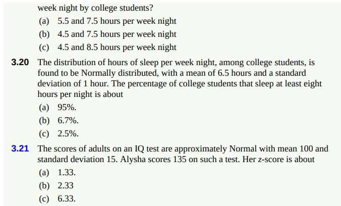
3.20 The distribution of hours of sleep per week night, among college students, is found to be Normally distributed, with a mean of 6.5 hours and a standard deviation of 1 hour. The percentage of college students that sleep at least eight hours per night is about (a) 95%. (b) 6.7%. (c) 2.5%.
3.19 The distribution of hours of sleep per week night, among college students, is found to be Normally distributed, with a mean of 6.5 hours and a standard deviation of 1 hour. What range contains the middle 95% of hours slept perweek night by college students? (a) 5.5 and 7.5 hours per week night
3.18 The standard deviation of the Normal distribution in Figure 3.15 is (a) 2. (b) 3. (c) 5. -8-6-4-2024 2 4 6 8 10 12
3.17 Figure 3.15 shows a Normal curve. The mean of this distribution is (a) 0. (b) 2. (c) 3.
3.16 To completely specify the shape of a Normal distribution, you must give (a) the mean and the standard deviation. (b) the five-number summary. (c) the median and the quartiles.
3.15 Which of these variables is most likely to have a Normal distribution? (a) Income per person for 150 different countries (b) Sale prices of 200 homes in Santa Barbara, California (c) Lengths of 100 newborns in Connecticut
3.14 The Medical College Admissions Test. A new version of the Medical College Admissions Test (MCAT) was introduced in spring 2015 and is intended to shift the focus from what applicants know to how well they can use what they know. One result of the change is that the scale on which the exam is
3.13 Table A. Use Table A to find the value z of a standard Normal variable that satisfies each of the following conditions. (Use the value of z from Table A that comes closest to satisfying the condition.) In each case, sketch a standard Normal curve with your value of z marked on the axis. (a)
3.12 APPLY YOUR KNOWLEDGE Use the Normal Table. Use Table A to find the proportion of observations from a standard Normal distribution that satisfies each of the following statements. In each case, sketch a standard Normal curve and shade the area under the curve that is the answer to the question.
3.11 Monsoon Rains. The summer monsoon rains in India follow approximately a Normal distribution with mean 852 millimeters (mm) of rainfall and standard deviation 82 mm. (a) In the drought year 1987, 697 mm of rain fell. In what percent of all years will India have 697 mm or less of monsoon rain?
3.10 Use the Normal Table. Use Table A to find the proportion of observations from a standard Normal distribution that satisfies each of the following statements. In each case, sketch a standard Normal curve and shade the area under the curve that is the answer to the question. (a) z < -0.42 (b) z>
3.9 Men's and Women's Heights. The heights of women aged 20-29 in the United States are approximately Normal with mean 64.2 inches and standard deviation 2.8 inches. Men the same age have mean height 69.4 inches with standard deviation 3.0 inches. What are the z-scores for a woman 5.5 feet tall and
3.8 SAT versus ACT. In 2015, when she was a high school senior, Linda scored 680 on the mathematics part of the SAT.5 The distribution of SAT math scores in 2015 was Normal with mean 511 and standard deviation 120. Jack took the ACT and scored 26 on the mathematics portion. ACT math scores for 2015
3.7 Monsoon Rains. The summer monsoon rains bring 80% of India's rainfall and are essential for the country's agriculture. Records going back more than a century show that the amount of monsoon rainfall varies from year to year according to a distribution that is approximately Normal with mean 852
3.6 Upper Arm Lengths. The upper arm length of males over 20 years old in the United States is approximately Normal with mean 39.1 centimeters (cm) and standard deviation 2.3 cm. Use the 68-95-99.7 rule to answer the following questions. (Start by making a sketch like Figure 3.10.) (a) What range
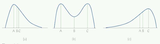
3.4 Mean and Median. Figure 3.7 displays three density curves, each with three points marked on it. At which of these points on each curve do the mean and the median fall? A BC A B C (a) (b) (c) A B C
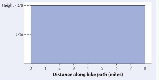
3.3 Mean, Median, and Quartiles. The density curve pictured in Figure 3.4 (on page 78) is called a uniform density. Because of the ease of computing areas under this density curve, it allows many computations to be done by hand. (a) What is the mean of the density curve pictured in Figure 3.4?
3.2 Accidents on a Bike Path. Examining the location of accidents on a level, 8- mile bike path shows that they occur uniformly along the length of the path. Figure 3.4 displays the density curve that describes the distribution of accidents. Height 1/8- 1/16-- 1 2 3 4 5 6 7 8 Distance along bike
3.1 Sketch Density Curves. Sketch density curves that describe distributions with the following shapes: (a) Symmetric, but with two peaks (that is, two strong clusters of observations) (b) Single peak and skewed to the left
2.53 Cholesterol for people in their 20s. Exercise 2.49 contains the cholesterol levels of individuals in their 20s from the NHANES survey in 2009-2010. The cholesterol levels are right-skewed, with a few large cholesterol levels. Which cholesterol levels are suspected outliers by the 1.5 IQR rule?
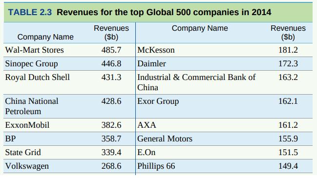
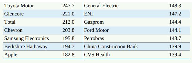
2.52 The Fortune Global 500. The Fortune Global 500, also known as the Global 500, is an annual ranking of the top 500 corporations worldwide as measured by revenue. In total, the Global 500 generated $31.2 trillion in revenues in 2014. Table 2.3 provides a list of the 30 companies with the highest
2.51 Shared pain and bonding. In Exercise 2.6, you should have noticed some low outliers in the pain group. BONDING (a) Compute the mean and the median of the bonding scores for the pain group, both with and without the two smallest scores. Do they have more of an effect on the mean or the median?
2.50 The changing face of America. Figure 1.10 (page 30) gives a stemplot of the percent of minority residents aged 18-34 in each of the 50 states and the District of Columbia. These data are given in Table 1.2. MINORITY(a) Give the five-number summary of this distribution. (b) Although there do
2.49 4step Cholesterol levels and age. The National Health and Nutrition Examination Survey (NHANES) is a unique survey that combines interviews and physical examinations.26 It includes basic demographic information; questions about topics such as diet, physical activity, and prescription
2.48 step Does playing video games improve surgical skill? In laparoscopic surgery, a video camera and several thin instruments are inserted into the patient's abdominal cavity. The surgeon uses the image from the video camera positioned inside the patient's body to perform the procedure by
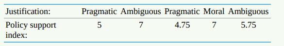
2.47 step Policy justification: Pragmatic vs. moral. How does a leader's justification of his/her organization's policy affect support for the policy? This study compared a moral, pragmatic, and ambiguous justification for three policy proposals: a politician's plan to fund a retirement planning
2.46 4step Do good smells bring good business? Businesses know that customers often respond to background music. Do they also respond to odors? Nicolas Guguen and his colleagues studied this question in a small pizza restaurant in France on Saturday evenings in May. On one evening, a relaxing
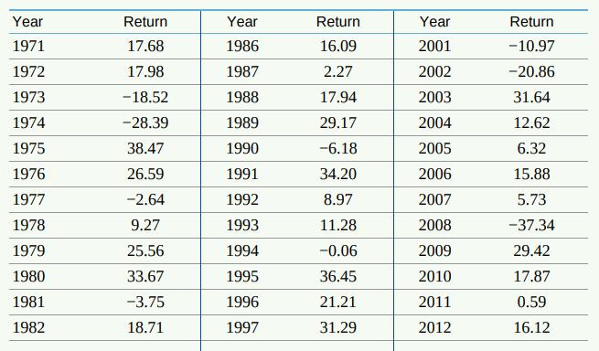
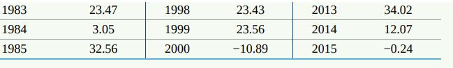
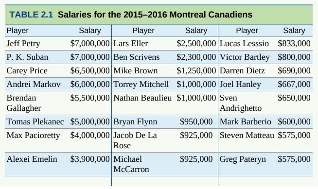
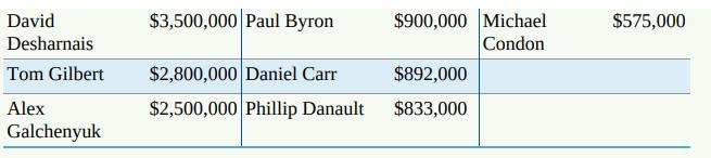
2.45 David Desharnais $3,500,000 Paul Byron $900,000 Michael Condon $575,000 Tom Gilbert $2,800,000 Daniel Carr $892,000 Alex Galchenyuk $2,500,000 Phillip Danault $833,000 Returns on stocks. How well have stocks done over the past generation? The Wilshire 5000 index describes the average
2.44 4step Athletes' salaries. The Montreal Canadiens were founded in 1909, and they are the longest continuously operating professional ice hockey team. The team has won 24 Stanley Cups, making them one of the most successful professional sports teams of the traditional four major sports of Canada
2.43 step Protective equipment and risk taking. Studies have shown that people who are using safety equipment when engaging in an activity tend to take increased risks. Will risk taking increase when people are not aware they are wearing protective equipment and are engaged in an activity that
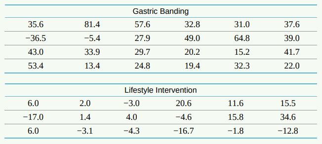
2.42 Adolescent obesity. Adolescent obesity is a serious health risk affecting more than 5 million young people in the United States alone. Laparoscopic adjustable gastric banding has the potential to provide a safe and effective treatment. Fifty adolescents between 14 and 18 years old with a body
2.41 You create the data. Give an example of a small set of data for which the mean is greater than the third quartile.
2.40 You create the data. Create a set of seven numbers (repeats allowed) that have the five-number summary Minimum = 4 Q = 8 M = 12 Q3 = 15 Maximum = 19 There is more than one set of seven numbers with this five-number summary. What must be true about the seven numbers to have this five-number
2.39 A standard deviation contest. This is a standard deviation contest. You must choose four numbers from the whole numbers 0 to 10, with repeats allowed.(a) Choose four numbers that have the smallest possible standard deviation. (b) Choose four numbers that have the largest possible standard
2.38 Thinking about means and medians. In 2014, approximately 2% of hourly rate workers were being paid at the federal minimum wage level. Would federal legislation to increase the minimum wage have a greater effect on the mean or the median income of all workers? Explain your answer.
2.37 Thinking about means. Table 1.2 (page 24) gives the percent of minority residents in each of the states. For the nation as a whole, 42.8% of residents are minorities. Find the mean of the 51 entries in Table 1.2. It is not 42.8%. Explain carefully why this happens. (Hint: The states with the
2.36 Never on Sunday: Also in Canada? Exercise 1.5 (page 20) gives the number of births in the United States on each day of the week during an entire year. The boxplots in Figure 2.6 are based on more detailed data from Toronto, Canada: the number of births on each of the 365 days in a year,
2.35 APPLET Behavior of the median. Place five observations on the line in the Mean and Median applet by clicking below it. (a) Add one additional observation without changing the median. Where is your new point? (b) Use the applet to convince yourself that when you add yet another observation
2.34 APPLET Making resistance visible. In the Mean and Median applet, place three observations on the line by clicking below it: two close together near the center of the line and one somewhat to the right of these two. (a) Pull the single rightmost observation out to the right. (Place the cursor
2.33 More on Nintendo and laparoscopic surgery. In Exercise 1.38 (page 42), you examined the improvement in times to complete a virtual gall bladder removal for those with and without four weeks of Nintendo WiiTM training. The most common methods for formal comparison of two groups use x and s to
2.32 Maternal age at childbirth. How old are women when they have their first child? Here is the distribution of the age of the mother for all firstborn children in the United States in 2014:17 Age Count Age Count 10-14 years 2,769 30-34 years 326,391 15-19 years 205,747 35-39 years 114,972 20-24
2.31 Guinea pig survival times. Here are the survival times in days of 72 guinea pigs after they were injected with infectious bacteria in a medical experiment." Survival times, whether of machines under stress or cancer patients after treatment, usually have distributions that are skewed to the
2.30 How much fruit do adolescent girls eat? Figure 1.14 (page 39) is a histogram of the number of servings of fruit per day claimed by 74 seventeen-year-old girls. (a) With a little care, you can find the median and the quartiles from the histogram. What are these numbers? How did you find them?
2.29 Comparing graduation rates. An alternative presentation to compare the graduation rates in Table 1.1 (page 22) by region of the country reports five- number summaries and uses boxplots to display the distributions. Do the boxplots fail to reveal any important information visible in the
2.28 Pulling wood apart. Exercise 1.46 (page 45) gives the breaking strengths of 20 pieces of Douglas fir. WOOD (a) Give the five-number summary of the distribution of breaking strengths. (b) Here is a stemplot of the data rounded to the nearest hundred pounds. The stems are thousands of pounds,
2.27 University endowments. The National Association of College and University Business Officers collects data on college endowments. In 2015, its report included the endowment values of 841 colleges and universities in the United States and Canada. When the endowment values are arranged in order,
2.26 Household assets. Once every three years, the Board of Governors of the Federal Reserve System collects data on household assets and liabilities through the Survey of Consumer Finances (SCF). 15 Here are some results from the 2013 survey. (a) Transaction accounts, which include checking,
2.25 Incomes of college grads. According to the U.S. Census Bureau's Current Population Survey, the mean and median 2014 income of people aged 25-34 years who had a bachelor's degree but no higher degree were $44,167 and $51,754, respectively. 14 Which of these numbers is the mean and which is the
2.24 Which of the following is most affected if an extreme high outlier is added to your data? (a) The median (b) The mean (c) The first quartile
2.23 The correct units for the standard deviation in Exercise 2.21 are (a) no units it's just a number. (b) pounds. (c) pounds squared.
2.22 What are all the values that a standard deviation s can possibly take? (a) 0s (b) 0s1 (c) -1s1
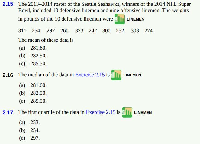
2.21 (a) all the individual observations. (b) the mean and the standard deviation. (c) the five-number summary. The standard deviation of the 10 weights in Exercise 2.15 (use your calculator)is about LINEMEN (a) 28.2. (b) 28.6. (c) 29.0.
2.20 To make a boxplot of a distribution, you must know
2.19 What percent of the observations in a distribution are greater than the first quartile? (a) 25% (b) 50% (c) 75%
2.18 If a distribution is skewed to the left, (a) the mean is less than the median. (b) the mean and median are equal. (c) the mean is greater than the median.
2.17 The first quartile of the data in Exercise 2.15 is LINEMEN (a) 253. (b) 254. (c) 297.
2.16 The median of the data in Exercise 2.15 is (a) 281.60. LINEMEN (b) 282.50. (c) 285.50.
2.15 The 2013-2014 roster of the Seattle Seahawks, winners of the 2014 NFL Super Bowl, included 10 defensive linemen and nine offensive linemen. The weights in pounds of the 10 defensive linemen were LINEMEN 311 254 297 260 323 242 300 252 303 274 The mean of these data is (a) 281.60. (b) 282.50.
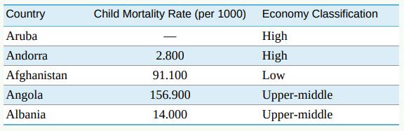
2.14 4step Worldwide Child Mortality. Although child mortality rates worldwide have dropped by more than 50% since 1990, it is still the case that 16,000 children under five years old die each day. The mortality rates for children under five vary from 1.9 per 1000 in Luxembourg to 156.9 per 1000 in
2.13 4step Logging in the Rain Forest. "Conservationists have despaired over destruction of tropical rain forest by logging, clearing, and burning." These words begin a report on a statistical study of the effects of logging in Borneo. Charles Cannon of Duke University and his coworkers compared
2.12 Choose a Summary. The shape of a distribution is a rough guide to whether the mean and standard deviation are a helpful summary of center and variability. For which of the following distributions would x and s be useful? In each case, give a reason for your decision. (a) Percents of high

Showing 5000 - 5100 of 8686

First
44
45
46
47
48
49
50
51
52
53
54
55
56
57
58
Last

Step by Step Answers

Services

Sitemap
Fun
Definitions
Become Tutor
Used Textbooks
Study Help Categories
Recent Questions
Expert Questions
Campus Wear
Sell Your Books

Company Info

Security
Copyrights
Privacy Policy
Terms & Conditions
SolutionInn Fee
Scholarship
Online Quiz
Give Feedback, Get Rewards

Get In Touch

About Us
Contact Us
Career
Jobs
FAQ
Student Discount
Campus Ambassador

Secure Payment

Download Our App

© 2026 SolutionInn. All Rights Reserved