New Semester Started Get 50% OFF Study Help! --h --m --s Claim Now

Question Answers

Textbooks

Find textbooks, questions and answers

Oops, something went wrong!

Change your search query and then try again

Result Not Found

Books FREE
Study Help
Tutors
AI Study Planner NEW
Sell Books

Search
Sign In
Register

study help
business
regression analysis

Introduction To Linear Regression Analysis 5th Edition Douglas C. Montgomery, Elizabeth A. Peck, G. Geoffrey Vining - Solutions

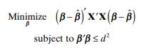
Show that the ridge estimator is the solution to the problem Minimize (B-B) x'x (B-B) B subject to B'
Consider the air pollution and mortality data given in Table B.15.a. Is there a problem with collinearity? Discuss how you arrived at this decision.b. Perform a ridge trace on these data.c. Select a k based upon the ridge trace from partb. Which estimates of the coeffi cients do you prefer for
Estimate the model parameters for the gasoline mileage data using principal -component regression.a. How much has the residual sum of squares increased compared to least squares?b. How much shrinkage in the coeffi cient vector has resulted?c. Compare the principal - component and ordinary ridge
Estimate model parameters for the Hald cement data (Table B.21) using principal - component regression.a. What is the loss in R2 for this model compared to least squares?b. How much shrinkage in the coeffi cient vector has resulted?c. Compare the principal - component model with the ordinary ridge
Estimate the parameters in a model for the gasoline mileage data in Table B.3 using ridge regression with the value of k determined by Eq. (9.8) . Does this model differ dramatically from the one developed in Problem 9.19?
Estimate the parameters in a model for the gasoline mileage data in Table B.3 using ridge regression.a. Use the ridge trace to select an appropriate value of k. Is the resulting model adequate?b. How much infl ation in the residual sum of squares has resulted from the use of ridge regression?c. How
Use ridge regression on the Hald cement data (Table B.21) using the value of k in Eq. (9.8) . Compare this value of k value selected by the ridge trace in Problem 9.17. Does the fi nal model differ greatly from the one in Problem 9.17?
Apply ridge regression to the Hald cement data in Table B.21.a. Use the ridge trace to select an appropriate value of k. Is the fi nal model a good one?b. How much infl ation in the residual sum of squares has resulted from the use of ridge regression?c. Compare the ridge · regression model with
The table below shows the condition indices and variance decomposition proportions for the acetylene data using centered regressors. Use this information to diagnose multicollinearity in the data and draw appropriate conclusions.Number Eigenvalue Condition Indices Variance Decomposition Proportions
Analyze the chemical process data in Table B.5 for evidence of multicollinearity. Use the variance infl ation factors and the condition number of X ′ X .
Analyze the housing price data in Table B.4 for multicollinearity. Use the variance infl ation factors and the condition number of X ′ X .
Use the gasoline mileage data in Table B.3 and compute the condition indices and variance - decomposition proportions, with the regressors centered. What statements can you make about multicollinearity in these data?
Using the gasoline mileage data in Table B.3 fi nd the eigenvectors associated with the smallest eigenvalues of X ′ X . Interpret the elements of these vectors.What can you say about the source of multicollinearity in these data?
Consider the gasoline mileage data in Table B.3.a. Does the correlation matrix give any indication of multicollinearity?b. Calculate the variance infl ation factors and the condition number of X ′ X .Is there any evidence of multicollinearity?
Use the regressors x2 (passing yardage), x7 (percentage of rushing plays), and x8(opponents ’ yards rushing) for the National Football League data in Table B.1.a. Does the correlation matrix give any indication of multicollinearity?b. Calculate the variance infl ation factors and the condition
Repeat Problem 9.4 without centering the regressors and compare the results.Which approach do you think is better?
Find the condition indices and the variance decomposition proportions for the Hald cement data (Table B.21), assuming centered regressors. What can you say about multicollinearity in these data?
Using the Hald cement data (Example 10.1), fi nd the eigenvector associated with the smallest eigenvalue of X ′ X . Interpret the elements of this vector.What can you say about the source of multicollinearity in these data?
Consider the Hald cement data in Table B.21.a. From the matrix of correlations between the regressors, would you suspect that multicollinearity is present?b. Calculate the variance infl ation factors.c. Find the eigenvalues of X ′ X .d. Find the condition number of X ′ X .
Consider the soft drink delivery time data in Example 3.1.a. Find the simple correlation between cases ( x1 ) an distance ( x2 ).b. Find the variance infl ation factors.c. Find the condition number of X ′ X . Is there evidence of multicollinearity in these data?
Consider the methanol oxidation data in Table B.20 . Perform a thorough analysis of these data. What conclusions do you draw from this analysis?
Consider the wine quality of young red wines data in Table B.19 . Regressor x1 is an indicator variable. Perform a thorough analysis of these data. What conclusions do you draw from this analysis?
Consider the fuel consumption data in Table B.18 . Regressor x1 is an indicator variable. Perform a thorough analysis of these data. What conclusions do you draw from this analysis?
Table B.17 contains hospital patient satisfaction data. Fit an appropriate regression model to the satisfaction response using age and severity as the regressors and account for the medical versus surgical classifi cation of each patient with an indicator variable. Has adding the indicator variable
Smith et al. [1992] discuss a study of the ozone layer over the Antarctic. These scientists developed a measure of the degree to which oceanic phytoplankton production is inhibited by exposure to ultraviolet radiation (UVB). The response is INHIBIT. The regressors are UVB and SURFACE, which is
Consider the life expectancy data given in Table B.16 . Create an indicator variable for gender. Perform a thorough analysis of the overall average life expectancy. Discuss the results of this analysis relative to your previous analyses of these data.
Using the wine quality data from Table B.11 , fi t a model relating wine quality y to fl avor x4 using region as an allocated code, taking on the values shown in the table (1,2,3). Discuss the interpretation of the parameters in this model. Compare the model to the one you built using indicator
Table B.11 presents data on the quality of Pinot Noir wine.a. Build a regression model relating quality y to fl avor x4 that incorporates the region information given in the last column. Does the region have an impact on wine quality?b. Perform a residual analysis for this model and comment on
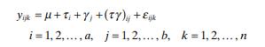
Two - Way Analysis of Variance. Suppose that two different sets of treatments are of interest. Let y ijk be the k th observation level i of the fi rst treatment type and level j of the second treatment type. The two - way analysis - of -variance model iswhere τ1 is the effect of level i of the fi
Montgomery [2009] presents an experiment concerning the tensile strength of synthetic fi ber used to make cloth for men ’ s shirts: The strength is thought to be affected by the percentage of cotton in the fi ber. The data are shown below.Percentage of Cotton Tensile Strength 15 7 7 15 11 9 20 12
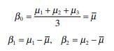
Alternate Coding Schemes for tbe Regression Approach to Analysis of Variance. Consider Eq. (8.18) , which represents the regression model corresponding to an analysis of variance with three treatments and n observations per treatment. Suppose that the indicator variables x1 and x2 are defi ned as
Suppose that a one - way analysis of variance involves four treatments but that a different number of observations (e.g., n i ) has been taken under each treatment. Assuming that n1 = 3, n2 = 2, n3 = 4, and n4 = 3, write down the y vector and X matrix for analyzing these data as a multiple
Continuation of Problem 8.7. Show how indicator variables can be used to develop a piecewise linear regression model with a discontinuity at the join point t.
Piecewise Linear Regression. In Example 7.3 we showed how a linear regression model with a change in slope at some point t ( xmin < t < xmax ) could be fi tted using splines. Develop a formulation of the piecewise linear regression model using indicator variables. Assume that the function is
Consider the National Football League data in Table B.1 . Build a linear regression model relating the number of games won to the yards gained rushing by opponents x8 , the percentage of rushing plays x7 , and a modifi cation of the turnover differential x5 . Specifi cally let the turnover
Consider the automobile gasoline mileage data in Table B.3 .a. Build a linear regression model relating gasoline mileage y to vehicle weight x10 and the type of transmission x11 . Does the type of transmission signifi cantly affect the mileage performance?b. Modify the model developed in part a to
Consider the automobile gasoline mileage data in Table B.3 .a. Build a linear regression model relating gasoline mileage y to engine displacement x1 and the type of transmission x11 . Does the type of transmission signifi cantly affect the mileage performance?b. Modify the model developed in part a
Consider the delivery time data in Example 3.1. In Section 4.2.5 noted that these observations were collected in four cities, San Diego, Boston, Austin, and Minneapolis.a. Develop a model that relates delivery time y to cases x1 , distance x2 , and the city in which the delivery was made. Estimate
Consider the regression models described in Example 8.4.a. Graph the response function associated with Eq. (8.10) .b. Graph the response function associated with Eq. (8.11) .
Consider the regression model (8.8) described in Example 8.3. Graph the response function for this model and indicate the role the model parameters play in determining the shape of this function.
Reconsider the data from Problem 7.21. Suppose that it is important to predict the response at the points x = 1750 and x = 1775.a. Find the predicted response at these points and the 95% prediction intervals for the future observed response at these points.b. Suppose that a fi rst - order model is
Below are data on y = green liquor (g/l) and x = paper machine speed(ft/min) from a kraft paper machine. (The data were read from a graph in an article in the Tappi Journal , March 1986.)y 16.0 15.8 15.6 15.5 14.8 x 1700 1720 1730 1740 1750 y 14.0 13.5 13.0 12.0 11.0 x 1760 1770 1780 1790 1795a.
Consider the solubility data from Problem 7.18. Suppose that a point of interest is x1 = 8.0, x2 = 3.0, and x3 = 5.0.a. For the quadratic model from Problem 7.18, predict the response at the point of interest and fi nd a 95% confi dence interval on the mean response at that point.b. Fit a model
Consider the quadratic regression model from Problem 7.18. Find the variance infl ation factors and comment on multicollinearity in this model.
An article in the Journal of Pharmaceutical Sciences ( 80 , 971 – 977, 1991) presents data on the observed mole fraction solubility of a solute at a constant temperature, along with x1 = dispersion partial solubility, x2 = dipolar partial solubility, and x3 = hydrogen bonding Hansen partial
Chemical and mechanical engineers often need to know the vapor pressure of water at various temperatures (the “ infamous ” steam tables can be used for this). Below are data on the vapor pressure of water ( y ) at various temperatures.Vapor Pressure, y(mmHg)Temperature, x( ° C)9.2 10 17.5 20
Consider the data in Problem 7.2.a. Fit a second - order model y = β0 + β1x + β11x2+ ε to the data. Evaluate the variance infl ation factors.b. Fit a second - order model y xx x =+ − ββ β 0 1 11 ( ) + − ( ) + ε 2 x to the data.Evaluate the variance infl ation factors.c. What can you
Consider the polynomial model in Problem 7.13. Find the variance infl ation factors and comment on multicollinearity in this model.
Modify the model in Problem 7.13 to investigate the possibility that a discontinuity exists in the regression function at x = 200 units. Estimate the parameters in this model. Test appropriate hypotheses to determine if the regression function has a change in both the slope and the intercept at x =
An operations research analyst is investigating the relationship between production lot size x and the average production cost per unit y . A study of recent operations provides the following data:x 100 120 140 160 180 200 220 240 260 280 300 y $9.73 9.61 8.15 6.98 5.87 4.98 5.09 4.79 4.02 4.46
Suppose that we wish to fi t a piecewise polynomial model with three segments: if x t2 , the polynomial is linear. Consider the modela. Does this segmented polynomial satisfy our requirements? If not, show how it can be modifi ed to do so.b. Show how the segmented model would be modifi ed to
Consider the patient satisfaction data in Section 3.6. Fit a complete second -order model to those data. Is there any indication that adding these terms to the model is necessary?
Consider the delivery time data in Example 3.1. Is there any indication that a complete second - order model in the two regressions cases and distance is preferable to the fi rst - order model in Example 3.1?
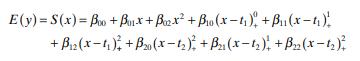
Suppose we wish to fi t the piecewise quadratic polynomial with a knot at x = t :Ey Sx x x x t x t x t ( ) = ( ) =+ + + − ( ) + − ( ) + − ( ) +++ ββ β β β β 00 01 02 2 10 011 112 2a. Show how to test the hypothesis that this quadratic spline model fi ts the data signifi cantly better
Consider the data in Problem 7.2.a. Fit a second - order model to these data using orthogonal polynomials.b. Suppose that we wish to investigate the addition of a third - order term to this model. Comment on the necessity of this additional term. Support your conclusions with an appropriate
Refer to Problem 7.6. Compute the residuals from the second - order model.Analyze the residuals and comment on the adequacy of the model.
The carbonation level of a soft drink beverage is affected by the temperature of the product and the fi ller operating pressure. Twelve observations were obtained and the resulting data are shown below.Carbonation, y Temperature, x1 Pressure, x2a. Fit a second - order polynomial.b. Test for signifi
Refer to Problem 7.4. Compute the residuals from the second - order model.Analyze the residuals and draw conclusions about the adequacy of the model.
Refer to Problem 7.2. Compute the residuals for the second - order model.Analyze the residuals and comment on the adequacy of the model.
A solid - fuel rocket propellant loses weight after it is produced. The following data are available Months since Production, x Weight Loss, y (kg)0.25 1.42 0.50 1.39 0.75 1.55 1.00 1.89 1.25 2.43 1.50 3.15 1.75 4.05 2.00 5.15 2.25 6.43 2.50 7.89a. Fit a second - order polynomial that expresses
Consider the values of x shown below:x = 1 0. , 0 1 70 1 25 1 20 1 45 1 85 1 60 1 50 1 95 2 00 . ,. ,. ,. ,. ,. ,. ,. ,.Suppose that we wish to fi t a second - order model using these levels for the regressor variable x. Calculate the correlation between x and x2. Do you see any potential diffi
Consider the methanol oxidation data in Table B.20. Perform a thorough infl uence analysis of these data. What conclusions do you draw from this analysis?
Consider the wine quality of young red wines data in Table B.19. For the purposes of this exercise, ignore regressor x1 . Perform a thorough infl uence analysis of these data. What conclusions do you draw from this analysis?
Consider the fuel consumption data in Table B.18. For the purposes of this exercise, ignore regressor x1 . Perform a thorough infl uence analysis of these data. What conclusions do you draw from this analysis?
Consider the patient satisfaction data in Table B.17. Fit a regression model to the satisfaction response using age and security as the predictors. Perform an infl uence analysis of the date and comment on your fi ndings.
For each model perform a thorough infl uence analysis of the life expectancy data given in Table B.16. Perform any appropriate transformations. Discuss your results.
Table B.14 contains data concerning the transient points of an electronic inverter. Fit a regression model to all 25 observations but only use x1 − x4 as the regressors. Investigate this model for infl uential observations and comment on your fi ndings.
Table B.13 contains data on the thrust of a jet turbine engine. Fit a regression model to these data using all of the regressors. Investigate this model for infl uential observations and comment on your fi ndings.
Table B.12 contains data collected on heat treating of gears. Fit a regression model to these data using all of the regressors. Investigate this model for infl uential observations and comment on your fi ndings.
Table B.11 contains data on the quality of Pinot Noir wine. Fit a regression model using clarity, aroma, body, fl avor, and oakiness as the regressors.Investigate this model for infl uential observations and comment on your fi ndings.
Formally show that COVRATIO S MS h i ip ii= ⎡⎣⎢ ⎤⎦⎥ −⎛⎝⎜ ⎞⎠⎟ ( )2 1 Res 1
Formally show that D r p h h i i ii ii = 1−
Perform a thorough infl uence analysis of kinematic viscosity data given in Table B.10. Perform any appropriate transformations. Discuss your results.
Perform a thorough infl uence analysis of the pressure drop data given in Table B.9. Perform any appropriate transformations. Discuss your results.
Perform a thorough infl uence analysis of the clathrate formation data given in Table B.8. Perform any appropriate transformations. Discuss your results.
Perform a thorough infl uence analysis of the oil extraction data given in Table B.7. Discuss your results.
Perform a thorough infl uence analysis of the NFL team performance data given in Table B.1. Discuss your results.
Perform a thorough infl uence analysis of the tube - fl ow reactor data given in Table B.6. Discuss your results.
Perform a thorough infl uence analysis of the Belle Ayr liquefaction runs given in Table B.5. Discuss your results.
Perform a thorough infl uence analysis of the property valuation data given in Table B.4. Discuss your results.
Perform a thorough infl uence analysis of the solar thermal energy test data given in Table B.2. Discuss your results.
French and Schultz ( “ Water Use Effi ciency of Wheat in a Mediterranean - type Environment, I The Relation between Yield, Water Use, and Climate, ” Australian Journal of Agricultural Research , 35 , 743 – 64) studied the impact of water use on the yield of wheat in Australia. The data below
A paper manufacturer studied the effect of three vat pressures on the strength of one of its products. Three batches of cellulose were selected at random from the inventory. The company made two production runs for each pressure setting from each batch. As a result, each batch produced a total of
A ceramic chemist studied the effect of four peak kiln temperatures on the density of bricks. Her test kiln could hold fi ve bricks at a time. Two samples, each from different peak temperatures, broke before she could test their density. The data follow. Perform the appropriate analysis.Temp.
A construction engineer studied the effect of mixing rate on the tensile strength of portland cement. From each batch she mixed, the engineer made four test samples. Of course, the mix rate was applied to the entire batch. The data follow. Perform the appropriate analysis.Mix Rate(rpm) Tensile
The fuel consumption data in Appendix B .18 is actually a subsampling problem. The batches of oil are divided into two. One batch went to the bus, and the other batch went to the truck. Perform the proper analysis of these data.
Consider the following subsampling model:y x i mj r ij = + ++ = ββ δε 0 1 i i ij ( ) 1 2,, , ,, , … … and = 1 2 (5.22)where m is the number of helicopters, r is the number of measured fl ight times for each helicopter, y ij is the fl ight time for the j th fl ight of the i th helicopter, x
Table B.14 contains data on the transient points of an electronic inverter.Delete the second observation and use x1 − x4 as regressors. Fit a multiple regression model to these data.a. Plot the ordinary residuals, the studentized residuals, and R - student versus the predicted response. Comment
Consider the model y X= + b e where E ( ε ) = 0 and Var( ε ) = σ2 V . Assume that V is known but not σ2. Show that( ′ − ′ ′ ( ) ′ ) ( ) − −− − − − yV y yV XXV X XV y 11 1 1 1 n p is an unbiased estimate of σ2.
Consider the model yX X = + 11 22 b be +where E ( ε) = 0 and Var( ε) = σ2 V . Assume that σ2 and V are known. Derive an appropriate test statistic for the hypotheses H H 02 12 : ,: b b = ≠ 0 0 Give the distribution under both the null and alternative hypotheses.
Suppose that we want to fi t the no - intercept model y = β x + ε using weighted least squares. Assume that the observations are uncorrelated but have unequal variances.a. Find a general formula for the weighted least - squares estimator of β .b. What is the variance of the weighted least -
Consider the simple linear regression model y i = β0 + β1x i + εi , where the variance of εi is proportional to xi 2, that is, Var( ) ε σ i i = x2 2.a. Suppose that we use the transformations y′ = y / x and x′ = l/ x . Is this a variance - stabilizing transformation?b. What are the
Schubert et al. ( “ The Catapult Problem: Enhanced Engineering Modeling Using Experimental Design, ” Quality Engineering , 4 , 463 – 473, 1992) conducted an experiment with a catapult to determine the effects of hook ( x1 ), arm length ( x2 ), start angle ( x3 ), and stop angle ( x4 ) on the
Vining and Myers ( “ Combining Taguchi and Response Surface Philosophies:A Dual Response Approach, ” Journal of Quality Technology , 22 , 15 – 22, 1990)analyze an experiment, which originally appeared in Box and Draper [ 1987 ].This experiment studied the effect of speed ( x1 ), pressure ( x2
Consider the kinematic viscosity data in Table B.10.a. Perform a thorough residual analysis of these data.b. Identify the most appropriate transformation for these data. Fit this model and repeat the residual analysis.
Consider the pressure drop data in Table B.9.a. Perform a thorough residual analysis of these data.b. Identify the most appropriate transformation for these data. Fit this model and repeat the residual analysis.
Consider the clathrate formation data in Table B.8.a. Perform a thorough residual analysis of these data.b. Identify the most appropriate transformation for these data. Fit this model and repeat the residual analysis.
Consider the three modelsa. y = β0 + β1 (1/ x ) + εb. 1/ y = β0 + β1 x + εc. y = x/ ( β0 − β1 x ) + εAll of these models can be linearized by reciprocal transformations. Sketch the behavior of y as a function of x . What observed characteristics in the scatter diagram would lead you to
Consider the methanol oxidation data in Table B.20. Perform a thorough analysis of these data. Recall the thorough residual analysis of these data from Exercise 4.29. Would a transformation improve this analysis? Why or why not? If yes, perform the transformation and repeat the full analysis.
Consider the fuel consumption data in Table B.18. For the purposes of this exercise, ignore regressor x1 . Recall the thorough residual analysis of these data from Exercise 4.27. Would a transformation improve this analysis? Why or why not? If yes, perform the transformation and repeat the full

Showing 900 - 1000 of 2175

First
3
4
5
6
7
8
9
10
11
12
13
14
15
16
17
Last

Step by Step Answers

Services

Sitemap
Fun
Definitions
Become Tutor
Used Textbooks
Study Help Categories
Recent Questions
Expert Questions
Campus Wear
Sell Your Books

Company Info

Security
Copyrights
Privacy Policy
Terms & Conditions
SolutionInn Fee
Scholarship
Online Quiz
Give Feedback, Get Rewards

Get In Touch

About Us
Contact Us
Career
Jobs
FAQ
Student Discount
Campus Ambassador

Secure Payment

Download Our App

© 2026 SolutionInn. All Rights Reserved