New Semester Started Get 50% OFF Study Help! --h --m --s Claim Now

Question Answers

Textbooks

Find textbooks, questions and answers

Oops, something went wrong!

Change your search query and then try again

Result Not Found

Books FREE
Study Help
Tutors
AI Study Planner NEW
Sell Books

Search
Sign In
Register

study help
business
regression analysis

Introduction To Linear Regression Analysis 5th Edition Douglas C. Montgomery, Elizabeth A. Peck, G. Geoffrey Vining - Solutions

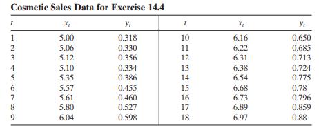
Consider the cosmetic sakes data in Exercise 14.4. Fit a time series regression model with autocorrected errors to these data. Compare this model with the results you obtained in Exercise 14.4 using the Cochrane – Orcutt procedure.
Consider the data in Exercise 14.3. Fit the lagged variables regression models shown in Eq. (14.26) and (14.27) to these data. Compare these models with the results you obtained in Exercise 14.3 using the Cochrane – Orcutt procedure, and with the time series regression model from Exercise 14.9.
Consider the data in Exercise 14.3. Fit a time series regression model with autocorrected errors to these data. Compare this model with the results you obtained in Exercise 14.3 using the Cochrane – Orcutt procedure.
Consider a simple linear regression model where time is the predictor variable. Assume that the errors are uncorrelated and have constant varianceσ2. Show that the variances of the model parameter estimates are V T T Tˆ ( )( ) β σ 0 2 22 1 1 ( ) = +−and VT Tˆ( ) β σ 1 2 212 1 ( ) = −
Consider the simple linear regression model y t = β0 + β1x + εt , where the error are generated by the second - order autoregressive processε ρε ρε t t tt =++ 11 22 − − a Discuss how the Cochrane – Orcutt iterative procedure could be used in this situation. What transformations would
Reconsider the data in Exercise 14.4. Defi ne a new set of transformed variables as the fi rst difference of the original variables, y yy t tt ′ = − −1 and x xx t tt ′ = − −1. Regress y′t on x′t through the origin. Compare the estimate of the slope from this fi rst - difference
The data in the following table gives the monthly sales for a cosmetics manufacturer ( y t ) and the corresponding monthly sales for the entire industry ( x t ). The units of both variables are millions of dollars.a. Build a simple linear regression model relating company sales to industry sales.
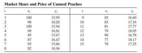
The data in the table below give the percentage share of market of a particular brand of canned peaches ( y t ) for the past 15 months and the relative selling price ( x t ).a. Fit a simple linear regression model to these data. Plot the residuals versus time. Is there any indication of
Table B.17 contains data on the global mean surface air temperature anomaly and the global CO 2 concentration. Fit a regression model to these data, using the global CO 2 concentration as the predictor. Analyze the residuals from this model. Is there evidence of autocorrelation in these data? If
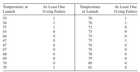
On 28 January 1986 the space shuttle Challenger was destroyed in an explosion shortly after launch from Cape Kennedy. The cause of the explosion was eventually identifi ed as catastrophic failure of the O - rings on the solid rocket booster. The failure likely occurred because the O - ring material
Reconsider the pneumoconiosis data in Table 13.1. Fit models using both the probit and complimentary log - log functions. Compare these models to the one obtained in Example 13.1 using the logit.
Consider the automobile purchase late in Problem 13.5. Fit models using both the probit and complementary log - log functions. Compare three models to the one obtained using the logit.
Consider a logistic regression model with a linear predictor that includes an interaction term, say x′β = β0 + β1x1 + β2x2 + β12x1x2 . Derive an expression for the odds ratio for the regressor x1 . Does this have the same interpretation as in the case where the linear predictor does not have
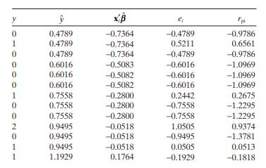
The table below shows the predicted values and deviance residuals for the Poisson regression model using x2 = bomb load as the regressor fi t to the aircraft damage data in Example 13.8. Plot the residuals and comment on model adequacy. y x pi 0 0.4789 -0.7364 -0.4789 -0.9786 1 0.4789 -0.7364
Reconsider the model for the drill data from Problem 13.16. Construct plots of the deviance residuals from the model and comment on these plots. Does the model appear satisfactory from a residual analysis viewpoint?
Reconsider the drill data from Problem 13.16. Fit a GLM using the log link and the gamma distribution, but expand the linear predictor to include all six of the two - factor interactions involving the four original regressors.Compare the model deviance for this model to the model deviance for
Reconsider the drill data from Problem 13.16. Remove any regressors from the original model that you think might be unimportant and rework parts b – e of Problem 13.16. Comment on your fi ndings.
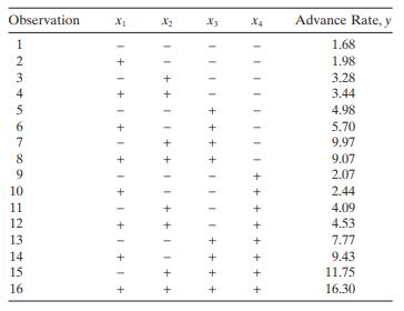
The data in the table below are from an experiment designed to study the advance rate y of a drill. The four design factors are x1 = load, x2 = fl ow, x3 = drilling speed, and x4 = type of drilling mud (the original experiment is described by Cuthbert Daniel in his 1976 book on industrial
The negative binomial probability mass function is f y y y , , π αααπ π α ( ) = + −−⎛⎝⎜ ⎞⎠⎟ ( ) − 1 11 for y = > 012 0 0 1 ,,, , … α π and ≤ ≤Show that the negative binomial is a member of the exponential family.
The exponential probability density function is fy e y y , , λλ λ λ ( ) = ≥ − for 0 Show that the exponential distribution is a member of the exponential family.
The gamma probability density function is f yr rey y ry r , , λ , λ λ λ ( ) = ( )≥ − −Γ1 for 0 Show that the gamma is a member of the exponential family.
Reconsider the model for the aircraft fastener data from Problem 13.3, parta. Construct plots of the deviance residuals from the model and comment on these plots. Does the model appear satisfactory from a residual analysis viewpoint?
Reconsider the model for the soft drink coupon data from Problem 13.4, parta. Construct plots of the deviance residuals from the model and comment on these plots. Does the model appear satisfactory from a residual analysis viewpoint?
Reconsider the model for the automobile purchase data from Problem 13.5, parta. Construct plots of the deviance residuals from the model and comment on these plots. Does the model appear satisfactory from a residual analysis viewpoint?
Reconsider the mine fracture data from Problems 13.7 and 13.8. Construct plots of the deviance residuals from the best model you found and comment on the plots. Does the model appear satisfactory from a residual analysis viewpoint?
Reconsider the mine fracture data from Problem 13.7. Remove any regressors from the original model that you think might be unimportant and rework parts b – e of Problem 13.7. Comment on your fi ndings.
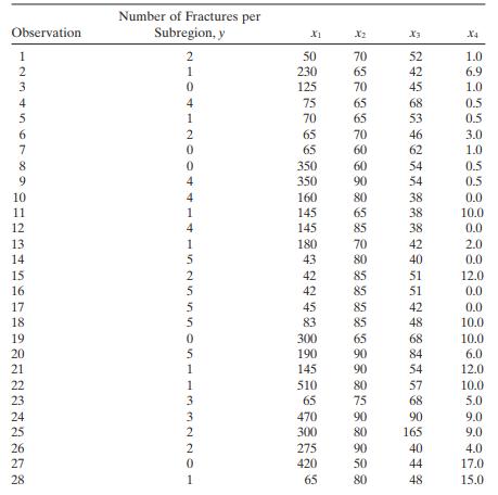
Myers [ 1990 ] presents data on the number of fractures ( y ) that occur in the upper seams of coal mines in the Appalachian region of western Virginia.Four regressors were reported: x1 = inner burden thickness (feet), the shortest distance between seam fl oor and the lower seam; x2 = percent
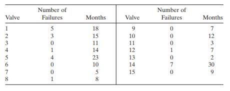
A chemical manufacturer has maintained records on the number of failures of a particular type of valve used in its processing unit and the length of time(months) since the valve was installed. The data are shown below.a. Fit a Poisson regression model to the data.b. Does the model deviance indicate
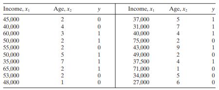
A study was performed to investigate new automobile purchases. A sample of 20 families was selected. Each family was surveyed to determine the age of their oldest vehicle and their total family income. A follow - up survey was conducted 6 months later to determine if they had actually purchased a
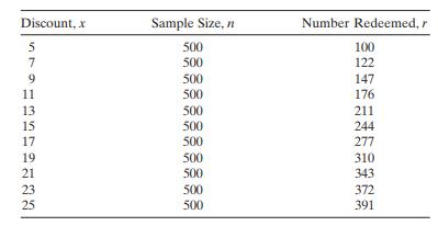
The market research department of a soft drink manufacturer is investigating the effectiveness of a price discount coupon on the purchase of a two -liter beverage product. A sample of 5500 customers was given coupons for varying price discounts between 5 and 25 cents. The response variable was the
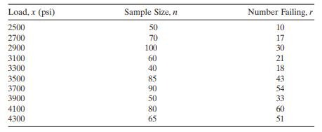
The compressive strength of an alloy fastener used in aircraft construction is being studied. Ten loads were selected over the range 2500 – 4300 psi and a number of fasteners were tested at those loads. The numbers of fasteners failing at each load were recorded. The complete test data are shown
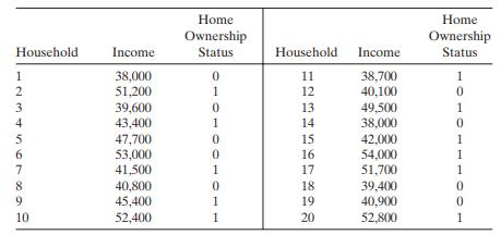
A study was conducted attempting to relate home ownership to family income. Twenty households were selected and family income was estimated, along with information concerning home ownership ( y = 1 indicates yes and y = 0 indicates no). The data are shown below.a. Fit a logistic regression model to
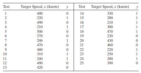
The table below presents the test - fi ring results for 25 surface - to - air antiaircraft missiles at targets of varying speed. The result of each test is either a hit ( y = 1) or a miss ( y = 0).a. Fit a logistic regression model to the response variable y . Use a simple linear regression model
The following data were collected on specifi c gravity and spectrophotometer analysis for 26 mixtures of NG (nitroglycerine), TA (triacetin), and 2 NDPA(2 - nitrodiphenylamine).There is a need to estimate activity coeffi cients from the model y xxx = + + = 1 βββ 11 12 33 εThe quantity
The following table gives the vapor pressure of water for various temperatures, previously reported in Exercise 5.2.a. Plot a scatter diagram. Does it seem likely that a straight - line model will be adequate?b. Fit the straight - line model. Compute the summary statistics and the residual plots.
Continuation of Problem 12.12. The two observations in each cell of the data table in Problem 12.12 are two replicates of the experiment. Each replicate was run from a unique batch of raw material. Fit the model yx x x = + θθ ε ( )( ) + θ θ43 1 1 2 2 3 where x3 = 0 if the observation comes
Continuation of Problem 12.12a. Fit the nonlinear model given in Problem 12.12 using the solution you obtained by linearizing the expectation function as the starting values.b. Test for signifi cance of regression. Does it appear that both variables x1 and x2 have important effects?c. Analyze the
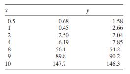
Consider the data below.These data were collected in an experiment where x1 = reaction time in minutes and x2 = temperature in degrees Celsius. The response variable y is concentration (grams per liter). The engineer is considering the model y xx = θ εa. Note that we can linearize the expectation
The data below represent the fraction of active chlorine in a chemical product as a function of time after manufacturinga. Construct a scatterplot of the data.b. Fit the Mitcherlich law (see Problem 12.10) to these data. Discuss how you obtained the starting values.c. Test for signifi cance of
Consider the model y e x =− + − θθ ε θ 1 2 3 This is called the Mitcherlich equation, and it is often used in chemical engineering. For example, y may be yield and x may be reaction time.a. Is this a nonlinear regression model?b. Discuss how you would obtain reasonable starting values of
Reconsider the data in the previous problem. The response measurements in the two columns were collected on two different days. Fit a new model yx e x =+ + θθ ε θ 32 1 2 1 to these data, where x1 is the original regressor from Problem 12.8 and x2 is an indicator variable with x2 = 0 if the
Consider the following observations:a. Fit the nonlinear regression model y e x = + θ ε θ 1 2 to these data. Discuss how you obtained the starting values.b. Test for signifi cance of regression.c. Estimate the error variance σ2 .d. Test the hypotheses H0 : θ1 = 0 and H0 : θ2 = 0. Are both
Reconsider the regression models in Problem 12.6, parts a –e. Suppose the error terms in these models were multiplicative, not additive. Rework the problem under this new assumption regarding the error structure.
For the models shown below, determine whether it is a linear model, an intrinsically linear model, or a nonlinear model. If the model is intrinsically linear, show how it can be linearized by a suitable transformation.a. y e x = + + θ ε θ θ 1 2 3b. y xx = + θθ θ ε + + θ 1 21 2 2 3c. y =
Consider the Gompertz model in Eq. (12.35) . Graph the expectation function for θ1 = 1, θ3 = 1, and θ2 1 8 = , 1, 8, 64 over the range 0 ≤ x ≤ 10.a. Discuss the behavior of the model as a function of θ2 .b. Discuss the behavior of the model as x → ∞ .c. What is E ( y ) when x = 0?
Sketch the expectation function for the logistic growth model (12.34) forθ1 = 1, θ3 = 1, and values of θ2 = 1, 4, 8, respectively. Overlay these plots on the same x – y axes. Discuss the effect of θ2 on the shape of the function.
Graph the expectation function for the logistic growth model (12.34) forθ1 = 10, θ2 = 2, and values of θ3 = 0.25, 1, 2, 3, respectively. Overlay these plots on the same set of x – y axes. What effect does the parameter θ3 have on the expectation function?
Consider the Michaelis – Menten model introduced in Eq. (12.23) . Graph the expectation function for θ1 = 100, 150, 200, 250 for θ2 = 0.06. Overlay these curves on the same set of x – y axes. What effect does the parameter θ1 have on the behavior of the expectation function?
Consider the Michaelis – Menten model introduced in Eq. (12.23) . Graph the expectation function for this model for θ1 = 200 and θ2 = 0.04, 0.06, 0.08, 0.10.Overlay these curves on the same set of x – y axes. What effect does the parameter θ2 have on the behavior of the expectation function?
Show that the least - squares estimate of β (say ˆb( )i ) with the i th observation deleted can be written in terms of the estimate based on all n points as e B = B-(XX)*x 1-h
If Z is the n × k matrix of standardized regressors and T is the k × k upper triangular matrix in Eq. (11.3) , show that the transformed regressors W = ZT− 1 are orthogonal and have unit variance.
Refer to Problem 11.2. Develop a model for the National Football League data using the prediction data set.a. How do the coeffi cients and estimated values compare with those quantities for the models developed from the estimation data?b. How well does this model predict the observations in the
Refer to Problem 11.2. What are the standard errors of the regression coeffi cients for the model developed from the estimation data? How do they compare with the standard errors for the model in Problem 3.5 developed using all the data?
PRESS statistics for two different models for the gasoline mileage data were calculated in Problems 11.6 and 11.7. On the basis of the PRESS statistics, which model do you think is the best predictor?
In Problem 3.6 a regression model was developed for the gasoline mileage data using the regressor vehicle length x8 and vehicle weight x10 . Calculate the PRESS statistic for this model. What conclusions can you draw about the potential performance of this model as a predictor?
In Problem 3.5 a regression model was developed for the gasoline mileage data using the regressor engine displacement x1 and number of carburetor barrels x6 . Calculate the PRESS statistic for this model. What conclusions can you draw about the model ’ s likely predictive performance?
Consider the delivery time data discussed in Example 11.3.a. Develop a regression model using the prediction data set.b. How do the estimates of the parameters in this model compare with those from the model developed from the estimation data? What does this imply about model validity?c. Use the
Consider the delivery time data discussed in Example 11.3. Find the PRESS statistic for the model developed from the estimation data. How well is the model likely to perform as a predictor? Compare this with the observed performance in prediction.
Calculate the PRESS statistic for the model developed from the estimation data in Problem 11.2. How well is the model likely to predict? Compare this indication of predictive performance with the actual performance observed in Problem 11.2.
Split the National Football League data used in Problem 3.1 into estimation and prediction data sets. Evaluate the statistical properties of these two data sets. Develop a model from the estimation data and evaluate its performance on the prediction data. Discuss the predictive performance of this
Consider the regression model developed for the National Football League data in Problem 3.1.a. Calculate the PRESS statistic for this model. What comments can you make about the likely predictive performance of this model?b. Delete half the observations (chosen at random), and refi t the
Use the all - possible - regressions selection on the methanol oxidation data in Table B.20 . Perform a thorough analysis of the best candidate models.Compare your results with stepwise regression. Thoroughly discuss your recommendations.
Use the all - possible - regressions selection on the wine quality of young red wines data in Table B.19 . Perform a thorough analysis of the best candidate models. Compare your results with stepwise regression. Thoroughly discuss your recommendations.
Use the all - possible - regressions selection on the fuel consumption data in Table B.18 . Perform a thorough analysis of the best candidate models.Compare your results with stepwise regression. Thoroughly discuss your recommendations.
Use the all - possible - regressions selection on the patient satisfaction data in Table B.17 . Perform a thorough analysis of the best candidate models.Compare your results with stepwise regression. Thoroughly discuss your recommendations.
Table B.15 presents data on air pollution and mortality. Use the all - possible -regressions selection on the air pollution data to fi nd appropriate models for these data. Perform a thorough analysis of the best candidate models.Compare your results with stepwise regression. Thoroughly discuss
Consider the Gorman and Toman asphalt data analyzed in Section 10.4.Recall that run is an indicator variable.a. Perform separate analyses of those data for run = 0 and run = 1.b. Compare and contrast the results of the two analyses from part a.c. Compare and contrast the results of the two analyses
Consider the electronic inverter data in Table B.14 . Delete observation 2 from the original data. Electrical engineering theory suggests that we should defi ne new variables as follows: y * = ln y , x x 1 1 1 * = , x x 2 2* = , x x 3 3 1 * = , and x x 4 4* = .a. Find an appropriate subset
Reconsider the electronic inverter data in Table B.14 . In Problems 10.24 and 10.25, you built regression models for the data using different variable selection algorithms. Suppose that you now learn that the second observation was incorrectly recorded and should be ignored.a. Fit a model to the
Compare the two best models that you have found in Problem 10.24 in terms of C p by calculating the confi dence intervals on the mean of the response for all points in the original data set. Based on a comparison of these confi -dence intervals, which model would you prefer? Now calculate the PRESS
Reconsider the electronic inverter data in Table B.14 . Use stepwise regression to fi nd an appropriate regression model for these data. Investigate model adequacy using residual plots. Compare this model with the one found by the all - possible - regressions approach in Problem 10.24.
Table B.14 presents data on the transient points of an electronic inverter.Use all possible regressions and the C p criterion to fi nd an appropriate regression model for these data. Investigate model adequacy using residual plots.
Compare the two best models that you have found in Problem 10.21 in terms of C p by calculating the confi dence intervals on the mean of the thrust response for all points in the original data set. Based on a comparison of these confi dence intervals, which model would you prefer? Now calculate the
Reconsider the jet turbine engine thrust data in Table B.13 . Use stepwise regression to fi nd an appropriate regression model for these data. Investigate model adequacy using residual plots. Compare this model with the one found by the all - possible - regressions approach in Problem 10.21.
Table B.13 presents data on the thrust of a jet turbine engine and six candidate regressors. Use all possible regressions and the C p criterion to fi nd an appropriate regression model for these data. Investigate model adequacy using residual plots.
Compare the models that you have found in Problems 10.17, 10.18, and 10.19 by calculating the confi dence intervals on the mean of the response PITCH for all points in the original data set. Based on a comparison of these confi -dence intervals, which model would you prefer? Now calculate the PRESS
Repeat Problem 10.17 using the two cross - product variables defi ned in Problem 10.18 as additional candidate regressors. Comment on the model that you fi nd.
Reconsider the heat treating data from Table B.12 . Fit a model to the PITCH response using the variables x SOAKTIME SOAKPCT x DIFFTIME DIFFPCT 1 2 = × =× and as regressors. How does this model compare to the one you found by the all - possible - regressions approach of Problem 10.17?
Table B.12 presents data on a heat treating process used to carburize gears.The thickness of the carburized layer is a critical factor in overall reliability of this component. The response variable y = PITCH is the result of a carbon analysis on the gear pitch for a cross - sectioned part. Use all
Rework Problem 10.14, parta, but exclude the region information.a. Comment on the difference in the models you have found. Is there indication that the region information substantially improves the model?b. Calculate confi dence intervals as mean quality for all points in the data set using the
Use the wine quality data in Table B.11 to construct a regression model for quality using the stepwise regression approach. Compare this model to the one you found in Problem 10.4, part a.
Table B.11 presents data on the quality of Pinot Noir wine.a. Build an appropriate regression model for quality y using the all -possible - regressions approach. Use C p as the model selection criterion, and incorporate the region information by using indicator variables.b. For the best two models
Suppose that the full model is y i = β0 + β1x i1 + β2x i2 + εi, i = 1, 2, . . . , n , where x i1 and x i2 have been coded so that S11 = S22 = 1. We will also consider fi tting a subset model, say y i = β0 + β1x i1 + εi .a. Let ˆ * β1 be the least - squares estimate of β1 from the full
Consider the all - possible - regressions analysis of the National Football League data in Problem 10.2. Identify the subset regression models that are R2 adequate (0.05).
Consider the all - possible - regressions analysis of Hald ’ s cement data in Example 10.1. If the objective is to develop a model to predict new observations, which equation would you recommend and why?
Analyze the air pollution and mortality data in Table B.15 using all possible regressions. Evaluate the subset models using the Rp 2, C p , and MSRes criteria.Justify your choice of the fi nal model using the standard checks for model adequacy.a. Use the all - possible - regressions approach to fi
Analyze the tube - fl ow reactor data in Table B.6 using all possible regre ssions.Evaluate the subset models using the Rp 2, C p , and MSRes criteria. Justify your choice of fi nal model using the standard checks for model adequacy.
Use the all - possible - regressions method to select a subset regression model for the Belle Ayr liquefaction data in Table B.5 . Evaluate the subset models using the C p criterion. Justify your choice of fi nal model using the standard checks for model adequacy.
Use stepwise regression with FIN = FOUT = 4.0 to fi nd the “ best ” set of regressor variables for the Belle Ayr liquefaction data in Table B.5 . Repeat the analysis with FIN = FOUT = 2.0. Are there any substantial differences in the models obtained?
Consider the property valuation data found in Table B.4 .a. Use the all - possible - regressions method to fi nd the “ best ” set of regressors.b. Use stepwise regression to select a subset regression model. Does this model agree with the one found in part a?
Consider the gasoline mileage performance data in Table B.3 .a. Use the all - possible - regressions approach to fi nd an appropriate regression model.b. Use stepwise regression to specify a subset regression model. Does this lead to the same model found in part a?
Consider the solar thermal energy test data in Table B.2 .a. Use forward selection to specify a subset regression model.b. Use backward elimination to specify a subset regression model.c. Use stepwise regression to specify a subset regression model.d. Apply all possible regressions to the data.
In stepwise regression, we specify that FIN ≥ FOUT (or tIN ≥ tOUT ). Justify this choice of cutoff values.
Consider the National Football League data in Table B.1 . Restricting your attention to regressors x1 (rushing yards), x2 (passing yards), x4 (fi eld goal percentage), x7 (percent rushing), x8 (opponents ’ rushing yards), and x9(opponents ’ passing yards), apply the all - possible - regressions
Consider the National Football League data in Table B.1 .a. Use the forward selection algorithm to select a subset regression model.b. Use the backward elimination algorithm to select a subset regression model.c. Use stepwise regression to select a subset regression model.d. Comment on the fi nal
Show that if X ′ X is in correlation form, Λ is the diagonal matrix of eigenvalues of X ′ X , and T is the corresponding matrix of eigenvectors, then the variance infl ation factors are the main diagonal elements of T Λ− 1 T ′ .
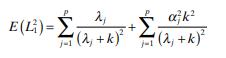
Consider the mean square error criterion for generalized ridge regression.Show that the mean square error is minimized by choosing kj j = σ α 2 2, j = 1, 2, . . . , p .
The mean square error criterion for ridge regression isTry to fi nd the value of k that minimizes E L1 2 ( ). What diffi culties are encountered? (1) - '(2,+k) 1-1 (+k)
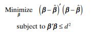
Show that the pure shrinkage estimator (Problem 9.25) is the solution to Minimize (B-B) (B-B) subject to B'
Pure Shrinkage Estimators (Stein [1960]) . The pure shrinkage estimator is defi ned as ˆ ˆ b b s = c , were 0 ≤ c ≤ 1 is a constant chosen by the analyst. Describe the kind of shrinkage that this estimator introduces, and compare it with the shrinkage that results from ridge regression.

Showing 800 - 900 of 2175

First
2
3
4
5
6
7
8
9
10
11
12
13
14
15
16
Last

Step by Step Answers

Services

Sitemap
Fun
Definitions
Become Tutor
Used Textbooks
Study Help Categories
Recent Questions
Expert Questions
Campus Wear
Sell Your Books

Company Info

Security
Copyrights
Privacy Policy
Terms & Conditions
SolutionInn Fee
Scholarship
Online Quiz
Give Feedback, Get Rewards

Get In Touch

About Us
Contact Us
Career
Jobs
FAQ
Student Discount
Campus Ambassador

Secure Payment

Download Our App

© 2026 SolutionInn. All Rights Reserved