New Semester
Started
Get
50% OFF
Study Help!
--h --m --s
Claim Now
Question Answers
Textbooks
Find textbooks, questions and answers
Oops, something went wrong!
Change your search query and then try again
S
Books
FREE
Study Help
Expert Questions
Accounting
General Management
Mathematics
Finance
Organizational Behaviour
Law
Physics
Operating System
Management Leadership
Sociology
Programming
Marketing
Database
Computer Network
Economics
Textbooks Solutions
Accounting
Managerial Accounting
Management Leadership
Cost Accounting
Statistics
Business Law
Corporate Finance
Finance
Economics
Auditing
Tutors
Online Tutors
Find a Tutor
Hire a Tutor
Become a Tutor
AI Tutor
AI Study Planner
NEW
Sell Books
Search
Search
Sign In
Register
study help
business
regression analysis
Achieve Business Analysis Certification: A Concise Guide To PMI-PBA®, CBAP® And CPRE Exam Successo The Channel City And Its Environs Pap/Psc Edition Klaus Nielsen (Author) - Solutions
Which two dimensions are used in the Thomas-Kilmann conflict mode model?a) Strengths and weaknessesb) Assertiveness and cooperativenessc) Power and conflictd) Collaboration and conflict
Which of these is not a typical type of requirement?a) Functional requirementb) Constraintsc) Quality requirementd) Risk-based requirement
Which of the following information would you not expect to find on a change request?a) Descriptionb) Priorityc) Titled) Title identifier
Sources and sinks help to identify the interfaces the system has with its environment. What is their relationship?a) Sources are outputs to the systems, while sinks are inputsb) Sources are inputs to the systems, while sinks are outputsc) Sources and sinks are both inputs to the system boundaryd)
The collect requirements process is important for tracking requirements. However, which of these is not an input?a) Scope management planb) Requirements management planc) Stakeholder management pland) Enterprise environmental factors
You are taking part in the process of developing the project charter. What is needed as input?a) Project statement of workb) Agreementsc) Enterprise environmental factorsd) All of the above
Total Quality Management (TQM) is described by four principles. Which of the following statements is a principle?a) Analysis of variabilityb) Management by factc) Learning and continuous improvementd) All of the above
Which of these prototypes is considered low fidelity?a) Old version or a competitive productb) Clickable versionc) Cardboard mockupd) A video of an acted screen
Which techniques are used in the control scope process?a) Variance analysisb) Expert judgmentc) Meetingsd) Change control tools
The process of tracking requirements is conducted in which PMI process(es)?a) The collect requirements and perform integrated change control processb) Perform integrated change control processc) Collect requirements processd) Verify scope process
According to Cockburn, of the choices below, what is the most effective form of communication?a) Paperb) Videotapec) Two people using a whiteboardd) Two people on the phone
Customers are primary stakeholders according to the Onion model, but which one of the following stakeholders would most likely be considered secondary?a) Employeesb) Suppliersc) Mediad) Communities
What is the overall purpose of supporting techniques?a) Help balance out the weaknesses and pitfalls of the selected elicitation techniqueb) Supporting techniques align stakeholdersc) Supporting techniques help spice up the techniques with video and layoutd) Additional documentation
The business analyst needs to analyze and communicate the solution’s identified gaps and deltas using quality assurance tools and methods in order to enable stakeholders to resolve discrepancies between:a) The project charter and the defined solutionb) The business case and the developed
Which one of the following factors most affects the choice of communication and collaboration technology?a) Costsb) Availability of technologyc) Project environmentd) Documentation
You are using the expert judgment technique to develop the project charter. Who would you consider as an expert?a) Only university professorsb) Subject matter expertsc) The PMOd) Everyone
What is meant when the status of a requirement is deleted?a) A special request was made by an authorized sourceb) An approved requirement has been canceled and removedc) A requirement was proposed, but it was not planned for implementationd) Work has been completed
Which one of these factors is not an advantage of brainstorming?a) Generates multiple ideas quicklyb) Involves multiple perspectivesc) Promotes equal participantsd) The true meaning may be misunderstood or ambiguous
A change in requirements most likely arises from:a) A planned changeb) Requirement errorsc) Changes in company strategyd) External stakeholder requirements
During stakeholder assessment, stakeholder salience is applied. Legitimacy and urgency has been measured, but what is missing?a) Probabilityb) Powerc) Relationshipsd) Concerns
What is osmotic communication?a) Communication around us which we pick upb) Nonverbal communicationc) Formal languaged) Personalized communication
Which of the following are not among the most commonly used traceability tools?a) Trace matricesb) Traceability chainc) Decision treesd) Specification trees
Which of the following is a property of a configuration of requirements?a) Testableb) Consistencyc) Transparentd) Objective
During the analyzing stakeholder process, stakeholder personalities are outlined. Which of the following techniques should not be used?a) MBTIb) Belbinc) Strength-based leadershipd) Porter’s five forces
Test-first development is a rapid XP cycle of testing, coding, and refactoring. It is reflected in the equation: test-first design + refactoring = ?a) Test behavior developmentb) Test driven developmentc) Software metricsd) Code reviews
Which one of these factors is not a disadvantage of survey techniques?a) Lack of access to committed stakeholdersb) Observation of nonverbal behaviorc) Documentation is subject to interpretationd) Conflicts are unresolved because people only understand their own point of view
The system boundary should be identified in order to do what?a) It is the system boundary that separates the system to be developed from its environmentb) It is the system boundary that separates the system to be developed and what is already developedc) It is the system boundary that separates the
Postrequirement specification traceability, which examines current or posterior artifacts, is also called:a) Backward traceabilityb) Forward traceabilityc) Prerequirement specification traceabilityd) Late requirement specification traceability
The future value is $8,000 in 4 years and the interest rate is 5%. What is the present value?a) $7,634.b) $6,775.c) $6,582.d) $8,575.
Why would the business analyst use a combination of different techniques for elicitation?a) To reduce costsb) To reduce timec) To reduce resourcesd) To minimize risk
Which of the following analyses are not used for change control?a) Impact change analysisb) Solution effect analysisc) Software impact analysisd) Impact configuration analysis
Which of the following activities is not typically part of configuration management?a) Configuration identificationb) Configuration status accountingc) Configuration verification and auditd) Configuration management analysis
‘U’ for User Satisfaction in PLUME criteria means:a) Ease of use and rememberingb) Time it takes to complete the tasksc) Subjective responses from usersd) Accuracy in carrying out the tasks
What are business rules used for?a) Define the rules that govern decisionsb) Define the rules that govern the teamc) Define the rules that govern the business cased) Define the rules that govern the project
Stakeholder analysis is performed to identify which of the following?a) Each stakeholder’s interest in the projectb) Potential conflicts in stakeholder viewpoint/interests that must be balancedc) Communication needs of each stakeholder throughout the phases of the projectd) All of the above
As a business analyst, what do you need to examine for prerequirement specification traceability (or backward traceability)?a) Legacy documentationb) Interviewsc) Shadowingd) Workshops with stakeholders
Which Scrum role determines how developing the solution will be accomplished?a) The Scrum Masterb) The project ownerc) The stakeholdersd) The development team
Which factor most influences the choice of elicitation techniques?a) The quality expectationsb) The business analyst’s lack of experience with a particular elicitation techniquec) Distinction between conscious, unconscious, and subconscious requirementsd) Opportunity of risks
What are the possible consequences of an incorrect or incomplete context analysis?a) Processes will not be documentedb) Some systems will not be in the scope statementc) Some systems will be missing while other systems will be wrongly includedd) Networks will not be documented
SMART criteria are short for:a) Specific, Measurable, Achievable, Relevant, and Testableb) Specific, Measurable, Achievable, Resource, and Time-boundc) Specific, Measurable, Achievable, Relevant, and Time-boundd) Specific, Manageable, Achievable, Relevant, and Time-bound
You are analyzing stakeholder values. Which of the following would you not include?a) Strategyb) Trustc) Collaborationd) Honesty
Some of the business analyst tasks with regard to traceability are:a) Collect requirement traceability informationb) Update requirement management planc) Communicate the updated traceability matrix to the stakeholdersd) All of the above
You need to elicit the Satisfiers from the Kano model. Which techniques would be most suitable?a) Survey techniquesb) Observationc) Creativity techniquesd) Document-centric techniques
Needs assessment translates business needs into:a) Goalsb) Scopec) Stakeholder needsd) A traceability matrix
Traceability is important because it has the ability to:a) Improve qualityb) Reduce riskc) Reduce development costd) All of the above
Incoming change requests received by the change control board can be classified as:a) Preventive requirement changeb) Corrective requirement changec) Internal changed) External change
If categorizing the requirement using the Kano model, what are the requirements users take for granted?a) Satisfiersb) Delightersc) Dissatisfiersd) None of the above
Possible influences of system contexts are processes; however, what kind of processes?a) Technical processesb) Physical processesc) Business processesd) All of the above
Which risk response/strategy is best for handling negative risks?a) Acceptanceb) Sharec) Avoidd) Enhance
Which of the following helps explain why a requirement has been changed?a) Traceabilityb) Testingc) Contract managementd) Scope management
What is the main task for the modifier at a change control board meeting?a) Receives the change requestb) Makes the final decisionc) Checks changes are made correctlyd) Implements the change
Using the Brown Cow Model, the current situation will be found in which section?a) Upper left cornerb) Lower left cornerc) Lower right cornerd) Upper right corner
Acceptance criteria are important because:a) They represent a specific and defined list of conditions that must be met before a project has been considered completed, and the project deliverables can and will be accepted by the businessb) They represent the stakeholder requirements to the defined
You are about to identify opportunities and challenges, and examine cost to the business of an upcoming project. Where would you likely find the answers?a) The budgetb) The business casec) The cost-benefit analysisd) The value proposition
Why is it important to document the life of the requirements?a) For lessons learnedb) For configuration management issuesc) It may assist in managing the budget and scheduled) It may help control scope
Requirements elicitation may derive from stakeholders (individuals or groups) and other sources.Which other sources?a) Legacy systemsb) System documentationc) Lessons learnedd) All of the above
Why is it important for the business analyst to define the system context?a) To know which systems are to be developedb) To know which systems are not includedc) Because the system context includes the constraintsd) Because the system context includes the systems attributes
You are waiting on a supplier to install a server. What kind of dependency is this?a) Mandatoryb) Discretionaryc) Externald) Internal
Which role is responsible for communicating the needs assessment in Scrum to the development team?a) The development teamb) The product ownerc) The Scrum Masterd) The business analyst
How does the business analyst ensure requirements are delivered as stated?a) Sign off on the contractb) Identify and analyze the requirementsc) Track requirementsd) Manage and monitor the requirements
What is one of the key challenges with requirements elicitation?a) Recording the voice of the customerb) Too many techniques to choose fromc) Too little timed) Managing scope
Which role would you not expect to take part in a change control board meeting?a) Quality assurance representativeb) Technical helpdeskc) Requirement engineerd) Configuration manager assistant
How does the business analyst ensure the delivered solution meets the business need?a) Validate the solutionb) Ensure signoffc) Verify the solutiond) Close project or phase
Which calculations would the business analyst most likely find in the cost-benefit section of the business case?a) Analog estimatesb) Return on investmentc) Risk analysisd) A budget
What is planguage?a) A key word oriented language for nonfunctional requirementsb) A software testing methodc) A key word oriented language for developing user storiesd) A feature-driven development language
The business analyst manages the life cycle of the requirements, which includes ongoing communication and collaboration with the stakeholders in order to:a) Manage, trace, and monitor the requirements throughout the life cycleb) Manage, trace, and monitor all constraints throughout the life cyclec)
During planning, the business analyst needs to take part in reviewing the business case and the project charter in order to ensure:a) Resources are allocatedb) A budget can be developedc) Objectives and goals are cleard) There is funding for the business case
The business analyst validates the solution and business needs with the use of:a) Acceptance criteriab) Software requirements specificationc) A traceability matrixd) Test cases
Negotiations: With whom are business analysts most likely to negotiate with often/daily?(The answer is found on page 271.)1 The project manager 2 The development team 3 The client 4 The PMO 5 Legal
Estimating Using Two Techniques: You are estimating activity for the business analysis plan and you are using your experience from earlier projects, which is similar to this one. In addition, you have access to data where you can measure the amount of work that can be done based upon available
Not Easy Reaching an Agreement: Your team is working on several options. Ten options are voted on and after multiple voting rounds where the option that gets the least votes is eliminated each round, one option is left standing and agreed upon. What technique has the team applied? (The answer is
Five Conflict Management Styles (Adkins, 2006): Read the following statements in Table 10.26 and rate each statement on a scale of 1 to 4—where 1 means rarely, 2 means sometimes, 3 means often, and 4 means always—indicating how likely you are to use the strategy listed in the right hand column.
Try This Presentation Technique: PechaKucha (2014) introduced a simple 20x20 format for slideshow presentations, where you present 20 slides, using 20 seconds per slide. The slides are changing automatically as you speak. Every presentation lasts for 6 minutes and 40 seconds
In-Sync Collaboration: Your team has focused on synchronous communication. Which of the following techniques would the team most likely apply? (The answer is found on page 271.)1 Facebook 2 Google docs 3 Voice calls 4 In-person meetings
Draw a Decision Tree: A Johannesburg farmer needs to make a decision. His orchard is expected to produce 200,000 bushels of peaches that he wishes to sell to a large grocery chain at $50 per bushel as Grade A peaches. However, he has great concern about the possibility of early frost damaging his
Match the Key Words to Their Definitions: Match the business analysis key words to their definitions. You will find the key words in Table 10.16 and the definitions in Table 10.17. You can use Table 10.18 to record your answers and determine your score. You will find the correct answers in Table
When working in agile, which two concepts are relevant in terms of evaluation?a) Test-driven development and definition of doneb) Behavior-driven development and software metricsc) Agile smells and refactoringd) Earned value management and validation
The plan-do-check-act cycle was developed by:a) Kaoru Ishikawab) Joseph Juranc) W. Edwards Demingd) None of the above
Which of these techniques is not used for quality management and control tools during evaluation?a) Process decision program chartsb) Prioritization matricesc) Tree diagramsd) Impact analysis
Which statistical quality control tools are used for identification?a) Control chartsb) Flowchartingc) Cause and effect diagramd) Histogram
When evaluating the deployed solution using valuation techniques, which one should not be used?a) Realisticb) Perceivedc) Normatived) Pessimistic
Match the Key Words to Their Definitions: Match the business analysis key words to their definitions. You will find the key words in Table 9.10, and their definitions in Table 9.11. You can use Table 9.12 to record your answers and determine your score. You will find the correct answers in Table
Decision Maker in Agile? In agile, who is the key decision maker when evaluating the deployed solution? (The answer is found on page 180.)1 The product owner 2 The Scrum Master 3 The development team 4 The steering committee 5 None of the above
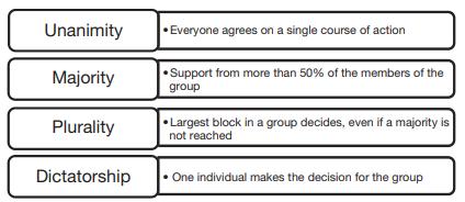
How to Use This at Work: In groups of two to four people, have participants list ways that they will use the materials presented in this section in their own work environments. Unanimity Majority Plurality Dictatorship Everyone agrees on a single course of action Support from more than 50% of the
Gaps: Which of the following techniques are helpful in analyzing solution gaps? (The answer is found on page 180.)1 Run charts 2 Tree diagrams 3 Statistical sampling 4 Forced field analysis 5 Matrix diagrams
Agile methodologies are based upon which development model?a) Spiralb) B-modelc) The waterfall modeld) V-model
The traceability tools are mostly:a) Specialized templatesb) Too expensive to usec) Difficult to used) For managing constraints
If a requirements status is proposed then it:a) Is an approved requirement that has been removedb) Has been requested by an authorized sourcec) Is a requirement that was proposed, but not planned for implementationd) Is work complete
Which development model is a variant of the waterfall model?a) V-modelb) B-modelc) Incremental development modeld) All of the above
If the project cycle is requirements definition, requirements validation, requirements documentation, and requirements management, which activity below is part of requirements management?a) Share datab) Test case automationc) Authoringd) Custom reports
Match the Key Words to Their Definitions: Match the business analysis key words to their definitions. You will find the key words in Table 8.22, and their definitions in Table 8.23. You can use Table 8.24 to record your answers and determine your score. You will find the correct answers in Table
Control Scope: Which of the following is an input to the control scope process? (The answer is found on page 166.)1 Variance analysis 2 Work performance information 3 Work performance data 4 Change requests
Update: You are in the process of updating Table 8.16. Which of the following items would you most likely see in the table? (The answers are found on page 166.)1 ID: 232 2 Name: Tyler Barnes 3 Description: Login 4 Life cycle: No 5 Stakeholders: Yes
Turn to Your Neighbor: If you are using this book in a study group or have a study buddy, discuss 2-3 main points you took away from this section.
Expert Judgment in Action: You are working on a building project and are in need of an expert when performing change control. Which of the following could be considered experts? (The answer is found on page 166.)1 An old university professor 2 Colleagues 3 A competitor on a similar project 4 The
Requirement elicitation is communication intensive and should be aligned with:a) The stakeholders’ needs and constraintsb) The business casec) The requirement management pland) The cost-benefit analysis
What makes elicitation difficult?a) Choosing the proper techniquesb) It requires close collaboration with the stakeholdersc) You hardly ever know when you are doned) Uncertain scope
The voice of the customers may be derived from?a) Customer complaintsb) Business rulesc) Impact analysisd) The business case
One approach to requirement elicitation on a high level is the Brown Cow Model in Figure 7.3.Which of these terms does it not contain?a) Pastb) Futurec) Howd) What
Which technique would you use to elicit requirements categorized in the Kano model as satisfiers?a) Observationb) Document-centric techniquesc) Both of the aboved) Survey techniques
Showing 200 - 300
of 2175
1
2
3
4
5
6
7
8
9
10
11
12
13
14
15
Last
Step by Step Answers