New Semester Started Get 50% OFF Study Help! --h --m --s Claim Now

Question Answers

Textbooks

Find textbooks, questions and answers

Oops, something went wrong!

Change your search query and then try again

Result Not Found

Books FREE
Study Help
Tutors
AI Study Planner NEW
Sell Books

Search
Sign In
Register

study help
business
regression analysis

Introduction To Linear Regression Analysis 6th Edition Douglas C. Montgomery, Elizabeth A. Peck, G. Geoffrey Vining - Solutions

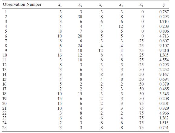
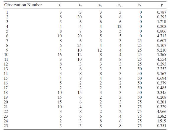
Table B. 14 presents data on the transient points of an electronic inverter. Fit a model to those data using an \(M\)-estimator. Is there an indication that observations might have been incorrectly recorded? Observation Number X1 X2 X3 Xs y 1234 3834 38 6 10 10 5862553 0 0.787 0 0.293 0 1.710
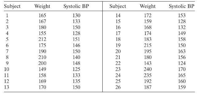
Consider the regression model in Problem 2.10 relating systolic blood pressure to weight. Suppose that we wish to predict an individual's weight given an observed value of systolic blood pressure. Can this be done using the procedure for predicting \(x\) given a value of \(y\) described in Section
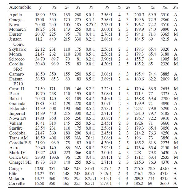
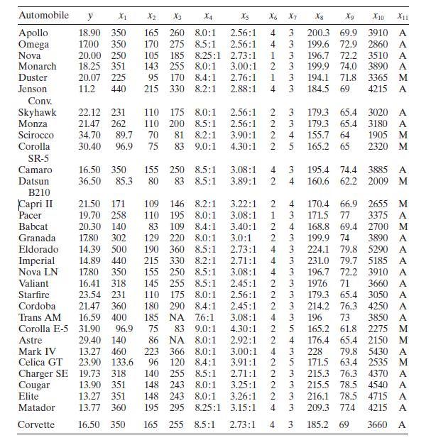
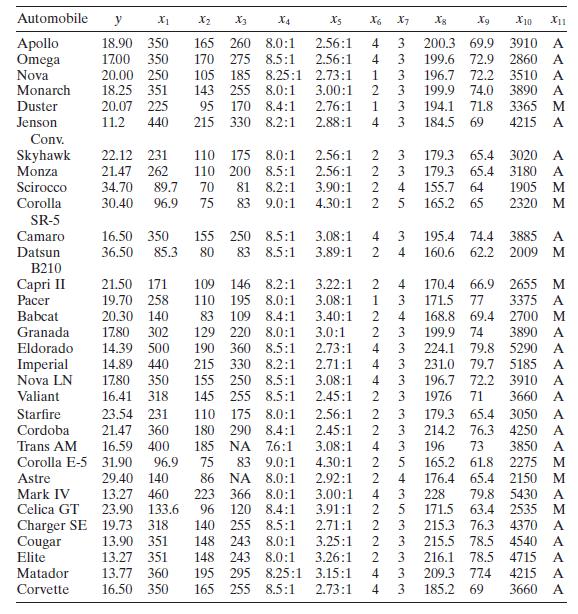
Consider the regression model in Problem 2.4 relating gasoline mileage to engine displacement.Data From Problem 2.4Table B. 3 presents data on the gasoline mileage performance of 32 different automobiles.a. If a particular car has an observed gasoline mileage of 17 miles per gallon, find a point
Consider a regression model relating total heat flux to radial deflection for the solar energy data in Table B.2.a. Suppose that the observed total heat flux is \(250 \mathrm{~kW}\). Find a point estimate of the corresponding radial deflection.b. Construct a \(90 \%\) confidence interval on radial
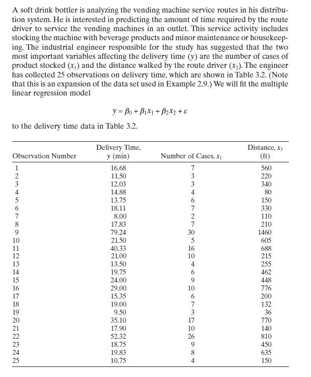
Consider the soft drink delivery time data in Example 3.1. Find an approximate \(95 \%\) bootstrap confidence interval on the regression coefficient for distance using \(m=1000\) bootstrap samples. Compare this to the usual normal-theory confidence interval.Example 3.1 A soft drink bottler is
Consider the soft drink delivery time data in Example 3.1. Find the bootstrap estimate of the standard deviation of \(\hat{\beta}_{1}\) using the following numbers of bootstrap samples: \(m=100, m=200, m=300, m=400\), and \(m=500\). Can you draw any conclusions about how many bootstrap samples are
Describe how you would find a bootstrap estimate of the standard deviation of the estimate of the mean response at a particular point, say \(\mathbf{x}_{0}\).
Describe how you would find an approximate bootstrap confidence interval on the mean response at a particular point, say \(\mathbf{x}_{0}\).
Consider the nonlinear regression model fit to the data in Problem 12.11. Find the bootstrap standard errors for the regression coefficients \(\hat{\theta}_{1}, \hat{\theta}_{2}\), and \(\hat{\theta}_{3}\) using \(m=1000\) bootstrap samples. Based on the results you obtain, comment on how the
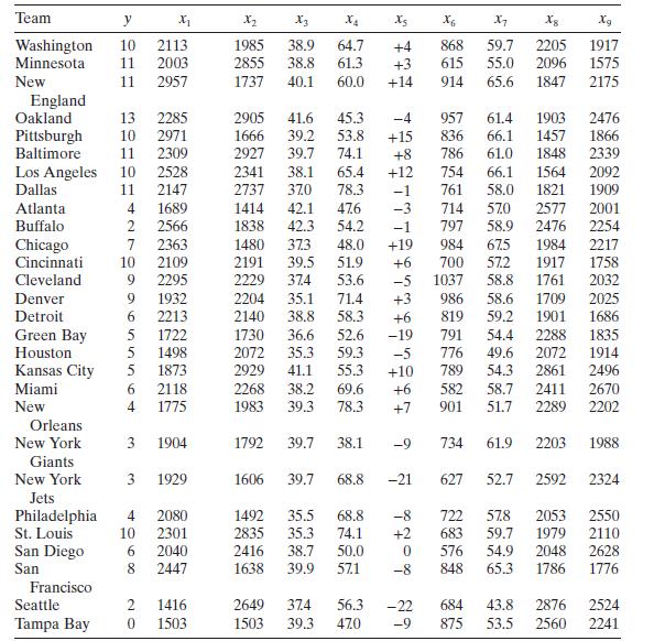
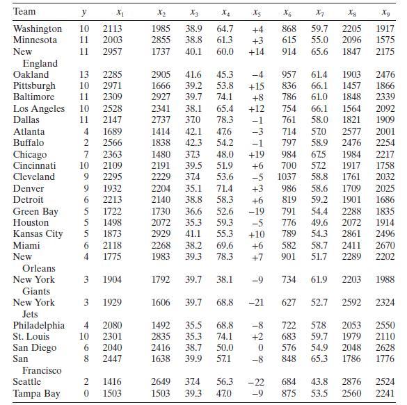
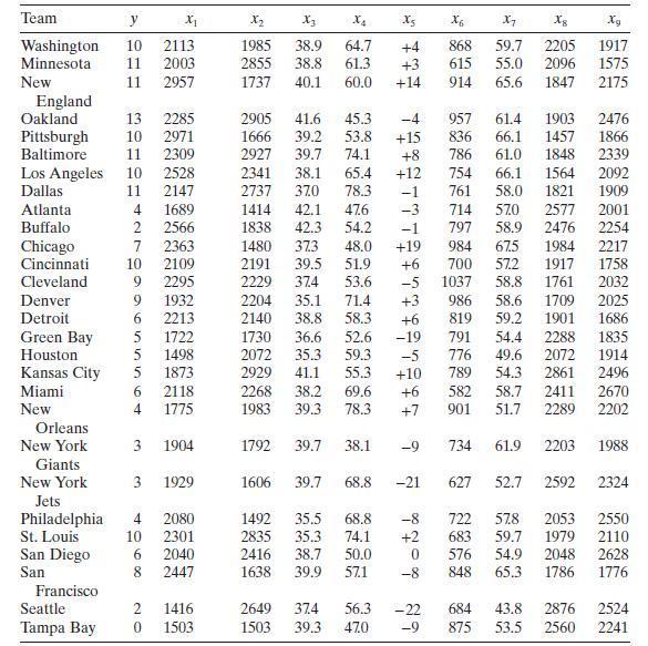
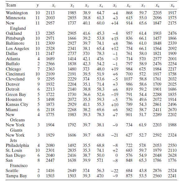
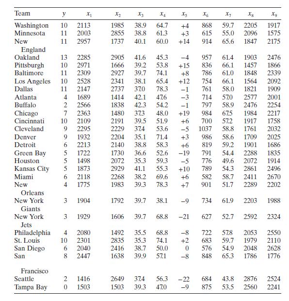
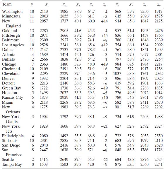
Consider the NFL team performance data in Table B.1. Construct a regression tree for this data set. Team y X2 X4 Xs X6 X7 Xg Xg Washington 10 2113 1985 38.9 64.7 +4 868 59.7 2205 1917 Minnesota 11 2003 2855 38.8 61.3 +3 615 55.0 2096 1575 New 11 2957 1737 40.1 60.0 +14 914 65.6 1847 2175 England
A Designed Experiment for Linear Regression. You wish to fit a simple linear regression model over the region \(-1 \leq x \leq 1\) using \(n=10\) observa-tions. Four experimental designs are under consideration: (i) 5 observations at \(x=-1\) and 5 observations at \(x=+1\), (ii) 4 observations at
An analyst is fitting a simple linear regression model with the objective of obtaining a minimum-variance estimate of the intercept \(\beta_{0}\). How should the data collection experiment be designed?
Suppose that you are fitting a simple linear regression model that will be used to predict the mean response at a particular point such as \(x_{0}\). How should the data collection experiment be designed so that a minimumvariance estimate of the mean of \(y\) at \(x_{0}\) is obtained?
Consider the linear regression model \(y=\beta_{0}+\beta_{1} x_{1}+\beta_{2} x_{2}+\varepsilon\), where the regressors have been coded so that\[\sum_{i=1}^{n} x_{i 1}=\sum_{i=1}^{n} x_{i 2}=0 \quad \text { and } \quad \sum_{i=1}^{n} x_{i 1}^{2}=\sum_{i=1}^{n} x_{i 2}^{2}=n\]a. Show that an
Suppose that you plan to run a \(2^{3}\) factorial experiment with 8 runs. You discover that your budget has been increased so that you can perform an additional 4 runs. Where would be the best places to run these additional 4 trials if you want to both get a model-independent estimate of error and
Continuation of Exercise 15.20. Suppose that a colleague suggests that you put the additional 4 runs at the center of the design region (assume that the three factors are continuous so that this is possible). What do you think about this suggestion? Does it improve the precision of estimation of
Suppose that you want to fit a first-order regression model with an interaction term to two continuous factors. You plan to conduct the experiment over the usual \(-1,+1\) region in both factors, but a physical constraint on the system limits the design region to \(x_{1}+x_{2} \geq 1.5\). You can
Consider the situation described in Exercise 15.22. Rework this problem assuming that the model you want to fit is second-order and you can afford to perform 12 runs.Data From Exercise 15.22Suppose that you want to fit a first-order regression model with an interaction term to two continuous
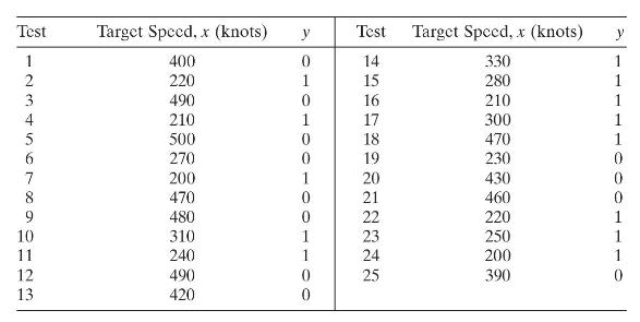
The table below presents the test-firing results for 25 surface-to-air antiaircraft missiles at targets of varying speed. The result of each test is either a hit \((y=1)\) or a miss \((y=0)\).a. Fit a logistic regression model to the response variable \(y\). Use a simple linear regression model as
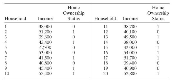
A study was conducted attempting to relate home ownership to family income. Twenty households were selected and family income was estimated, along with information concerning home ownership ( \(y=1\) indicates yes and \(y=0\) indicates no). The data are shown below.a. Fit a logistic regression
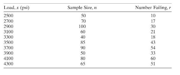
The compressive strength of an alloy fastener used in aircraft construction is being studied. Ten loads were selected over the range \(2500-4300\) psi and a number of fasteners were tested at those loads. The numbers of fasteners failing at each load were recorded. The complete test data are shown
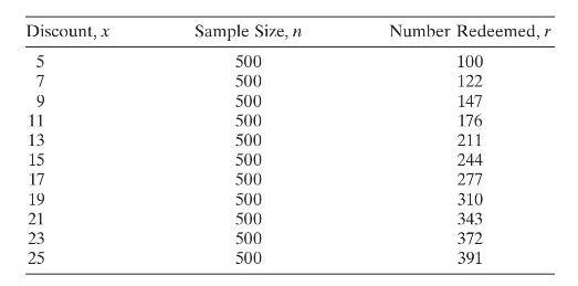
The market research department of a soft drink manufacturer is investigating the effectiveness of a price discount coupon on the purchase of a twoliter beverage product. A sample of 5500 customers was given coupons for varying price discounts between 5 and 25 cents. The response variable was the
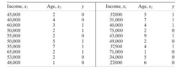
A study was performed to investigate new automobile purchases. A sample f 20 families was selected. Each family was surveyed to determine the age of their oldest vehicle and their total family income. A follow-up survey was conducted 6 months later to determine if they had actually purchased a new
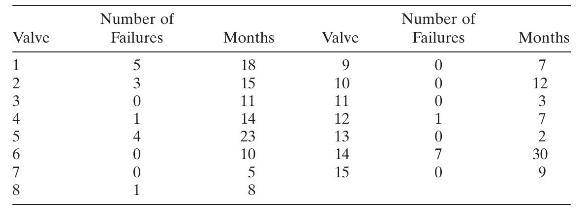
A chemical manufacturer has maintained records on the number of failures of a particular type of valve used in its processing unit and the length of time (months) since the valve was installed. The data are shown below.a. Fit a Poisson regression model to the data.b. Does the model deviance
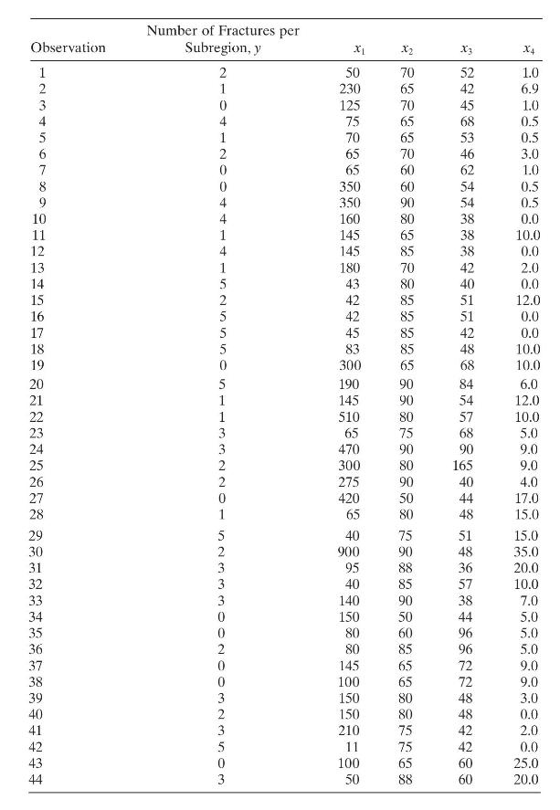
Myers [1990] presents data on the number of fractures (y) that occur in the upper seams of coal mines in the Appalachian region of western Virginia. Four regressors were reported: \(x_{1}=\) inner burden thickness (feet), the shortest distance between seam floor and the lower seam; \(x_{2}=\)
Reconsider the model for the soft drink coupon data from Problem 13.4, part a. Construct plots of the deviance residuals from the model and comment on these plots. Does the model appear satisfactory from a residual analysis viewpoint?Problem 13.4The market research department of a soft drink
Reconsider the model for the aircraft fastener data from Problem 13.3, part a. Construct plots of the deviance residuals from the model and comment on these plots. Does the model appear satisfactory from a residual analysis viewpoint?Problem 13.3The compressive strength of an alloy fastener used
The gamma probability density function is\[f(y, r, \lambda)=\frac{\lambda^{r}}{\Gamma(r)} e^{-\lambda y} y^{r-1} \quad \text { for } y, \lambda \geq 0\]Show that the gamma is a member of the exponential family.
The exponential probability density function is\[f(y, \lambda)=\lambda e^{-\lambda y} \quad \text { for } y, \lambda \geq 0\]Show that the exponential distribution is a member of the exponential family.
The negative binomial probability mass function is\[\begin{aligned}& \qquad f(y, \pi, \alpha)=\left(\begin{array}{c}y+\alpha-1 \\\alpha-1\end{array}\right) \pi^{\alpha}(1-\pi)^{y} \\& \text { for } y=0,1,2, \ldots, \alpha>0 \text { and } 0 \leq \pi \leq 1\end{aligned}\]Show that the negative
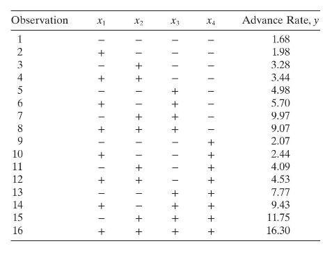
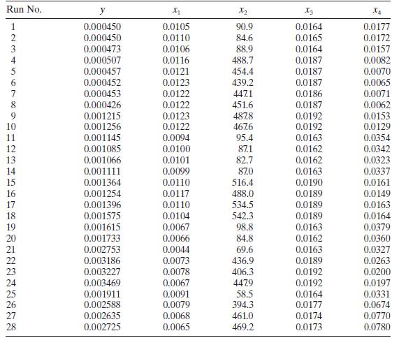
The data in the table below are from an experiment designed to study the advance rate \(y\) of a drill. The four design factors are \(x_{1}=\) load, \(x_{2}=\) flow, \(x_{3}=\) drilling speed, and \(x_{4}=\) type of drilling mud (the original experiment is described by Cuthbert Daniel in his 1976
Reconsider the drill data from Problem 13.16. Remove any regressors from the original model that you think might be unimportant and rework parts b-e of Problem 13.16. Comment on your findings.Data From Problem 13.16The data in the table below are from an experiment designed to study the advance
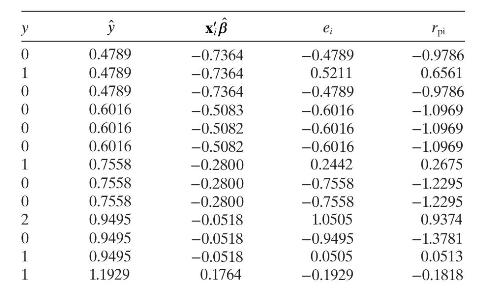
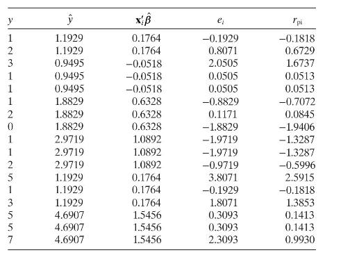
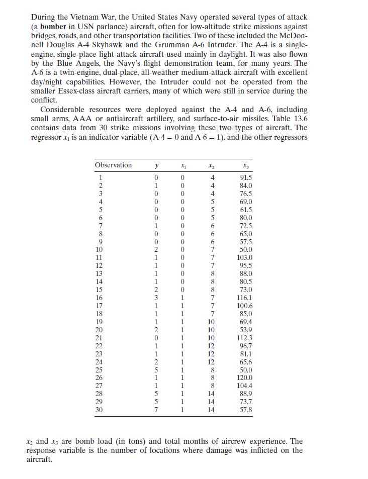
The table below shows the predicted values and deviance residuals for the Poisson regression model using \(x_{2}=\) bomb load as the regressor fit to the aircraft damage data in Example 13.8. Plot the residuals and comment on model adequacy.Example 13.8 y x B ei "pi 0 0.4789 -0.7364 -0.4789
Consider a logistic regression model with a linear predictor that includes an interaction term, say \(\mathbf{x}^{\prime} \boldsymbol{\beta}=\beta_{0}+\beta_{1} x_{1}+\beta_{2} x_{2}+\beta_{12} x_{1} x_{2}\). Derive an expression for the odds ratio for the regressor \(x_{1}\). Does this have the
The theory of maximum-likelihood states that the estimated large-sample covariance for maximum-likelihood estimates is the inverse of the information matrix, where the elements of the information matrix are the negatives of the expected values of the second partial derivatives of the log-likelihood
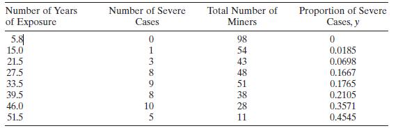
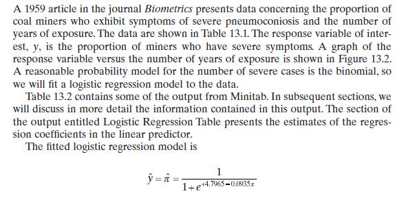
Reconsider the pneumoconiosis data in Table 13.1. Fit models using both the probit and complimentary log-log functions. Compare these models to the one obtained in Example 13.1 using the logit.Table 13.1Example 13.1 Number of Years of Exposure Number of Severe Cases Total Number of Miners
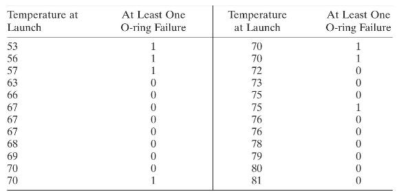
On 28 January 1986 the space shuttle Challenger was destroyed in an explosion shortly after launch from Cape Kennedy. The cause of the explosion was eventually identified as catastrophic failure of the O-rings on the solid rocket booster. The failure likely occurred because the O-ring material was
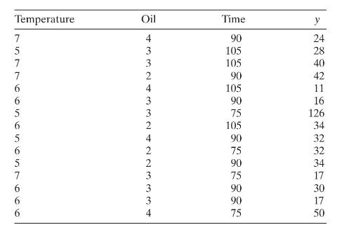
A student conducted a project looking at the impact of popping temperature, amount of oil, and the popping time on the number of inedible kernels of popcorn. The data follow. Analyze these data using Poisson regression. Temperature Oil Time y 4 33243324223334 755466565655666 90
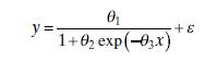
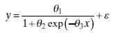
Sketch the expectation function for the logistic growth model (12.34) for \(\theta_{1}=1, \theta_{3}=1\), and values of \(\theta_{2}=1,4,8\), respectively. Overlay these plots on the same \(x-y\) axes. Discuss the effect of \(\theta_{2}\) on the shape of the function.Equation (12.34) y= 01 1+0
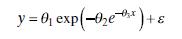
Consider the Gompertz model in Eq. (12.35). Graph the expectation function for \(\theta_{1}=1, \theta_{3}=1\), and \(\theta_{2}=\frac{1}{8}, 1,8,64\) over the range \(0 \leq x \leq 10\).Equation (12.35)a. Discuss the behavior of the model as a function of \(\theta_{2}\).b. Discuss the behavior of
For the models shown below, determine whether it is a linear model, an intrinsically linear model, or a nonlinear model. If the model is intrinsically linear, show how it can be linearized by a suitable transformation.a. \(y=\theta_{1} e^{\theta_{2}+\theta_{3} x}+\varepsilon\)b.
Reconsider the regression models in Problem 12.6, parts a-e. Suppose the error terms in these models were multiplicative, not additive. Rework the problem under this new assumption regarding the error structure.Data From Problem 12.6For the models shown below, determine whether it is a linear
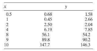
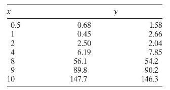
Consider the following observations:a. Fit the nonlinear regression model\[y=\theta_{1} e^{\theta_{2} x}+\varepsilon\]to these data. Discuss how you obtained the starting values.b. Test for significance of regression.c. Estimate the error variance \(\sigma^{2}\).d. Test the hypotheses \(H_{0}:
Reconsider the data in the previous problem. The response measurements in the two columns were collected on two different days. Fit a new model\[y=\theta_{3} x_{2}+\theta_{1} e^{\theta_{2} x_{1}}+\varepsilon\]to these data, where \(x_{1}\) is the original regressor from Problem 12.8 and \(x_{2}\)
Consider the model\[y=\theta_{1}-\theta_{2} e^{-\theta_{3} x}+\varepsilon\]This is called the Mitcherlich equation, and it is often used in chemical engineering. For example, \(y\) may be yield and \(x\) may be reaction time.a. Is this a nonlinear regression model?b. Discuss how you would obtain
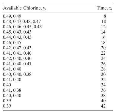
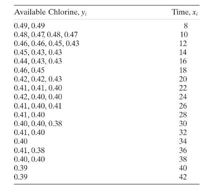
The data below represent the fraction of active chlorine in a chemical product as a function of time after manufacturing.a. Construct a scatterplot of the data.b. Fit the Mitcherlich law (see Problem 12.10) to these data. Discuss how you obtained the starting values.Data From Problenc. Test for
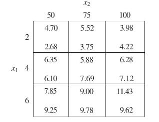
Consider the data below.These data were collected in an experiment where \(x_{1}=\) reaction time in minutes and \(x_{2}=\) temperature in degrees Celsius. The response variable \(y\) is concentration (grams per liter). The engineer is considering the
The following table gives the vapor pressure of water for various temperatures, previously reported in Exercise 5.2.Exercise 5.2The following table gives the vapor pressure of water for various temperaturesa. Plot a scatter diagram. Does it seem likely that a straight-line model will be adequate?b.
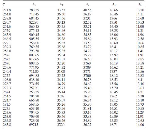
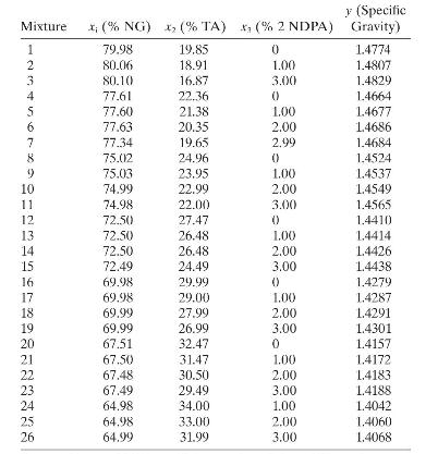
The following data were collected on specific gravity and spectrophotometer analysis for 26 mixtures of NG (nitroglycerine), TA (triacetin), and 2 NDPA (2-nitrodiphenylamine).There is a need to estimate activity coefficients from the model\[y=\frac{1}{\beta_{1} x_{1}+\beta_{1} x_{2}+\beta_{3}
A major problem associated with many mining projects is subsidence, or sinking of the ground above the excavation. The mining engineer needs to control the amount and distribution of this subsidence. This will ensure that structures on the surface survive the excavation. There are several factors
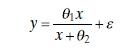
In the field of ecology, the relationship between the concentration of available dissolved organic substrate and the rate of uptake (velocity) of that substrate by heterotrophic microbial communities has been described by the Michaelis-Menten model. The velocity \((y)\) and concentration \((x)\)
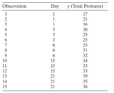
In a study to develop the growth behavior for protozoa colonization in a particular lake, an experiment was conducted in which 15 sponges were placed in a lake and 3 sponges at a time were gathered. Then the number of protozoa were counted at 1, 3, 6, 15, and 21 days. In this case the
The following data were collected on specific gravity and spectrophotometer analysis for 26 mixtures of NG (nitroglycerine), TA (triacetin and 2 NDPA (2-nitrodiphenylamine).There is a need to estimate activity coefficients from the model\[y=\frac{1}{\beta_{1} x_{1}+\beta_{1} x_{2}+\beta_{3}
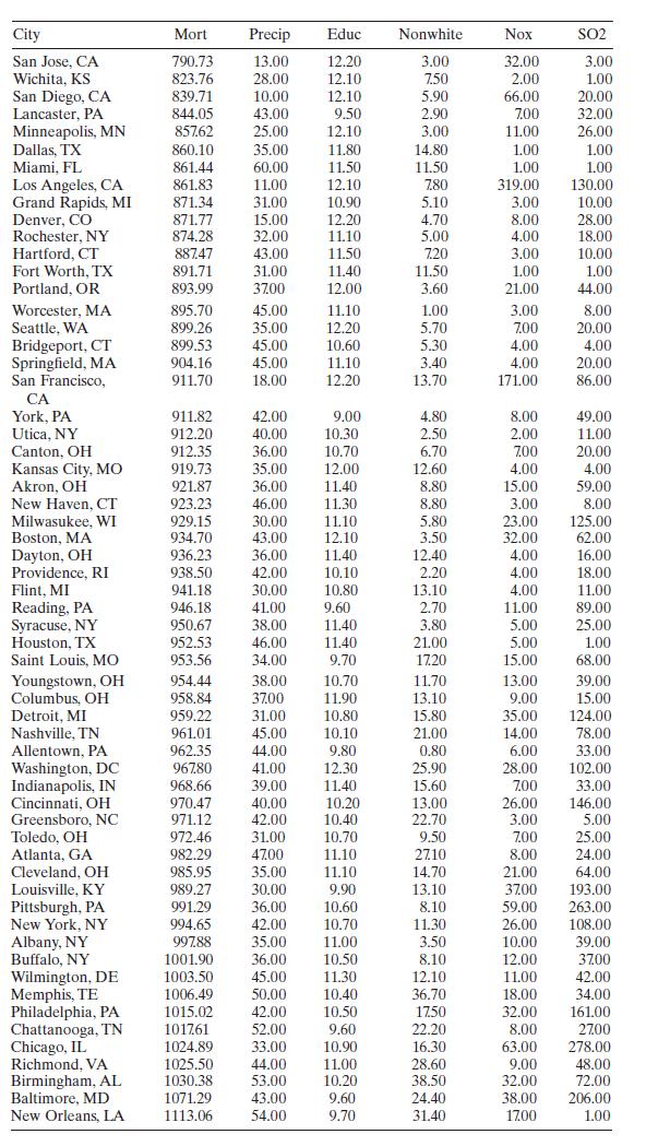
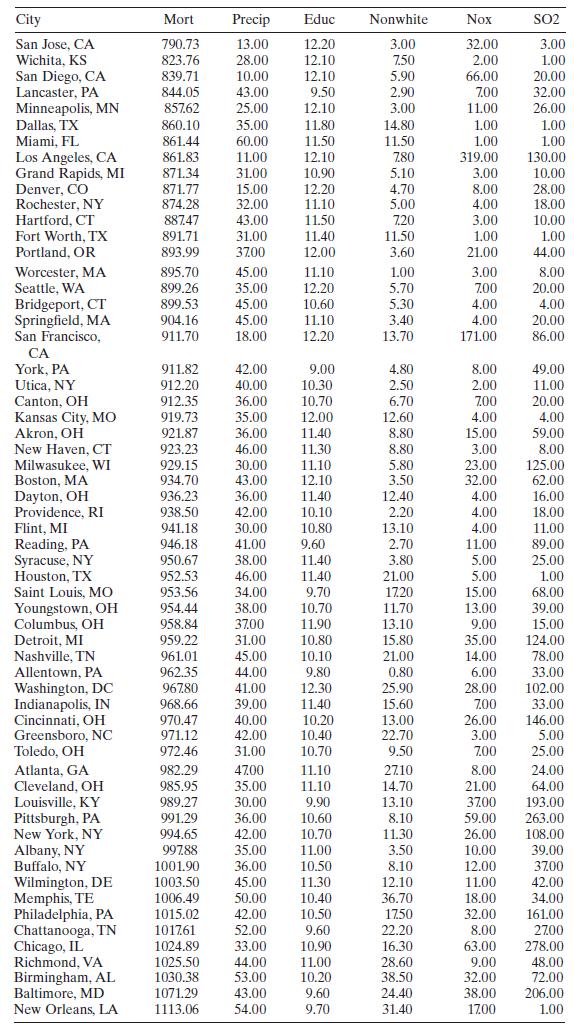
Table B. 15 presents data on air pollution and mortality. Use the all-possibleregressions selection on the air pollution data to find appropriate models for these data. Perform a thorough analysis of the best candidate models. Compare your results with stepwise regression. Thoroughly discuss your
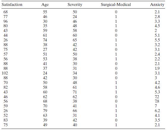
Use the all-possible-regressions selection on the patient satisfaction data in Table B.17. Perform a thorough analysis of the best candidate models. Compare your results with stepwise regression. Thoroughly discuss your recommendations. Satisfaction Age Severity Surgical-Medical Anxiety 8788928 68
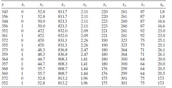
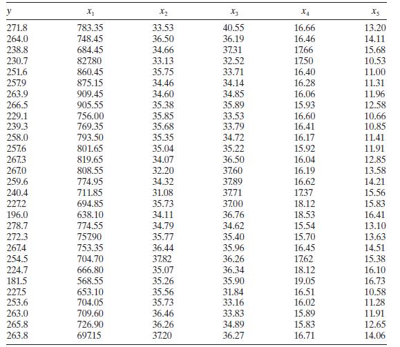
Use the all-possible-regressions selection on the fuel consumption data in Table B.18. Perform a thorough analysis of the best candidate models. Compare your results with stepwise regression. Thoroughly discuss your recommendations. y X2 X3 X4 X6 1 8 343 0 52.8 811.7 2.11 220 261 87 1.8 356 1 52.8
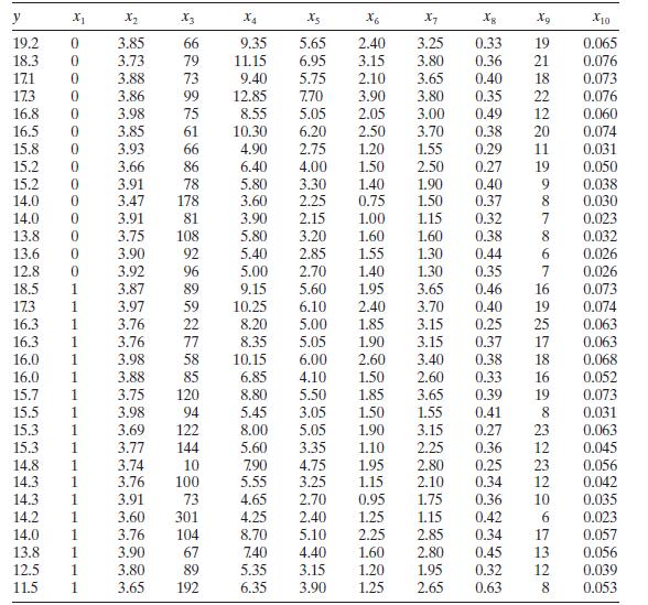
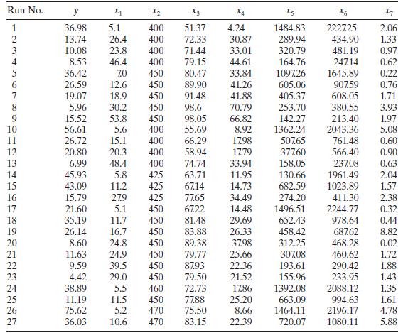
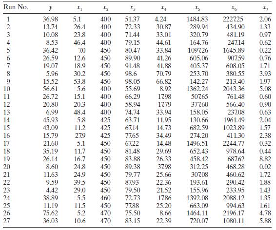
Use the all-possible-regressions selection on the wine quality of young red wines data in Table B.19. Perform a thorough analysis of the best candidate models. Compare your results with stepwise regression. Thoroughly discuss your recommendations. y X2 X3 X4 X5 X6 X7 Xg 10 19.2 0 3.85 66 9.35
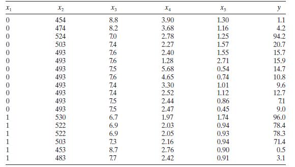
Use the all-possible-regressions selection on the methanol oxidation data in Table B.20. Perform a thorough analysis of the best candidate models. Compare your results with stepwise regression. Thoroughly discuss your recommendations. x1 x2 X3 x4 Xs y 0 454 8.8 3.90 1.30 1.1 0 474 8.2 3.68 1.16 4.2
Generalized Regression Techniques and Variable Selection In Chapter 9, we introduced generalized regression techniques as an approach to handling the multicollinearity problem. The LASSO can sometimes be used effectively for variable selection because it can shrink some regression coefficients to
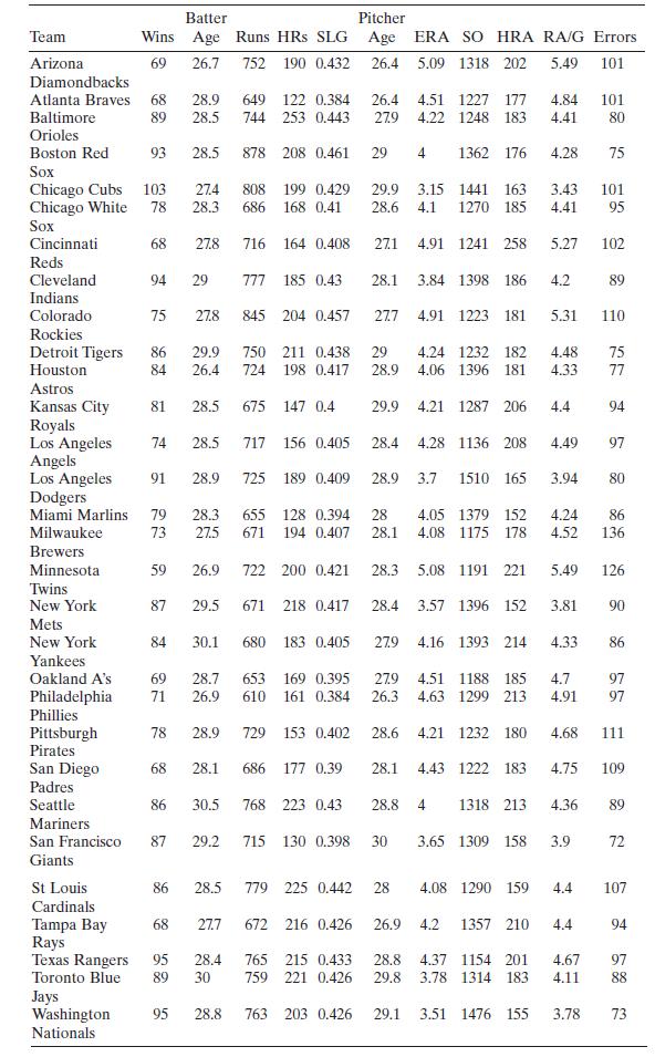
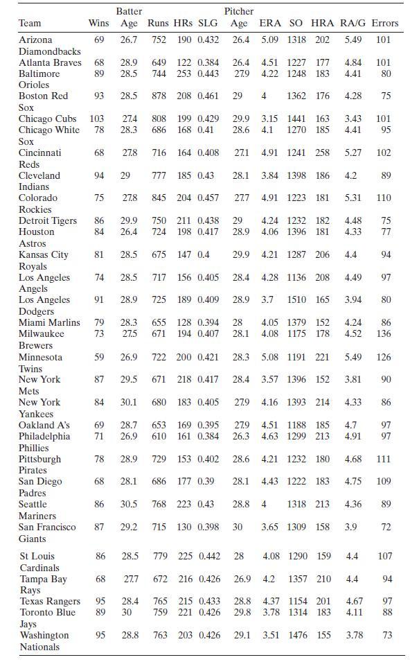
Table B. 22 contains data on 1916 team performance for Major League Baseball. Use all possible regressions to build a model for this data. Perform a residual analysis on the final model and comment on model adequacy. Team Batter Pitcher Wins Age Runs HRS SLG Age ERA SO HRA RA/G Errors Arizona 69
Use stepwise regression to build a model for the 1916 MLB team performance data in Table B.22. Perform a residual analysis on the final model. Compare this model to the all possible regressions model from Problem 10.36.Data From Problem 36Table B. 22 contains data on 1916 team performance for Major
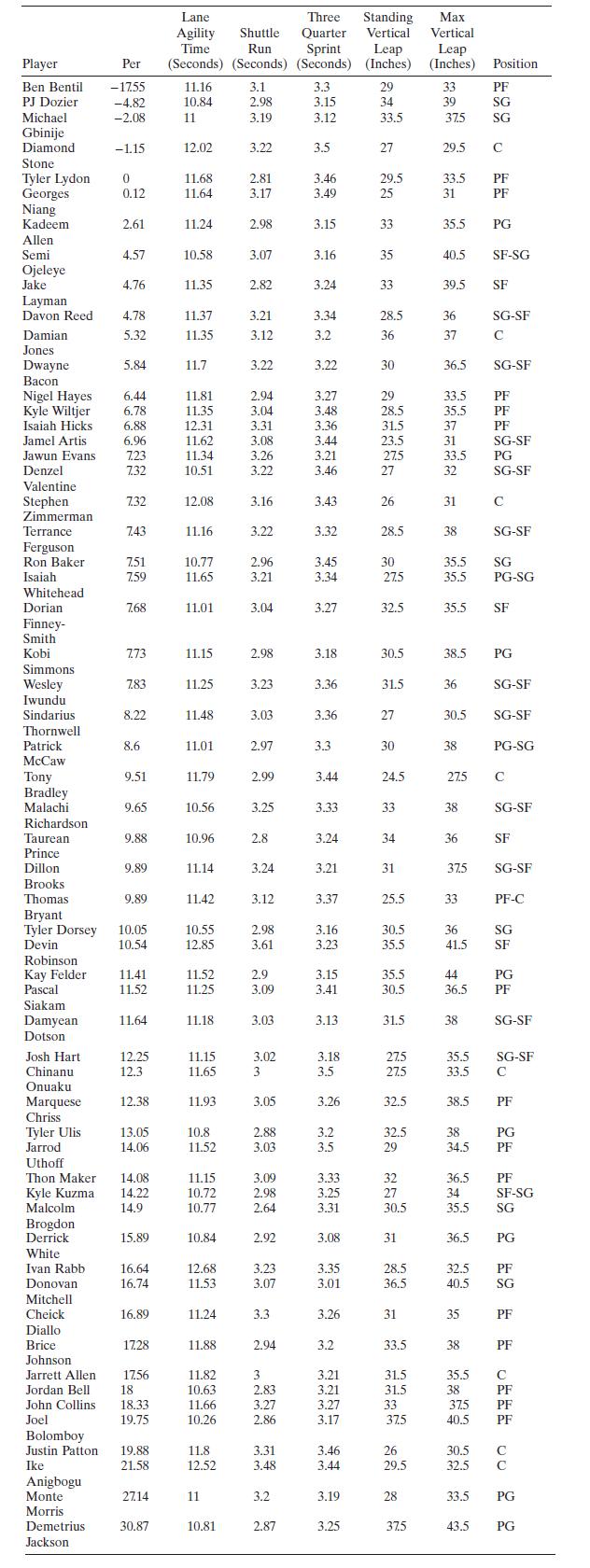
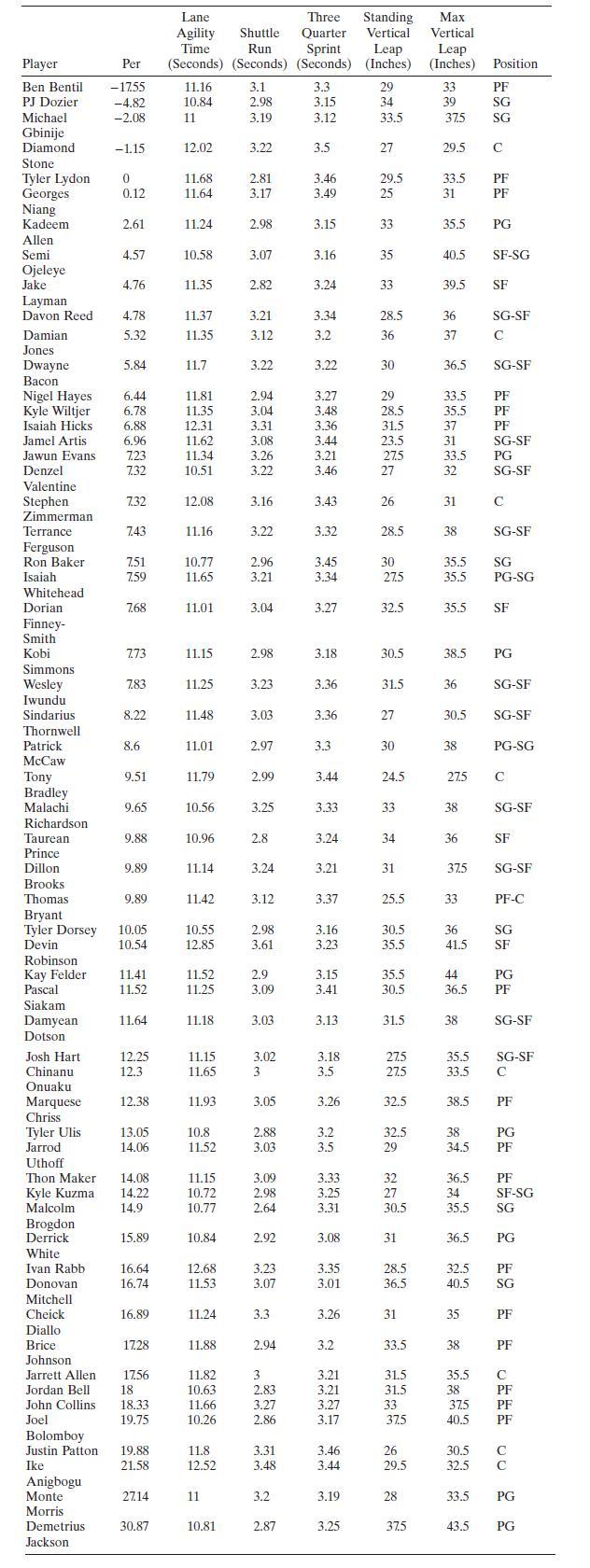
Table B. 23 contains data from the NBA Combine. Use all possible regressions to build a model for these data. Perform a residual analysis on the final model and comment on model adequacy. Time Run Player Per Ben Bentil -1755 11.16 3.1 3.3 PJ Dozier -4.82 10.84 2.98 Michael -2.08 11 3.19 Gbinije
Use stepwise regression to build a model for the NBA Combine data in Table B.23. Perform a residual analysis on the final model. Compare this model to the all possible regressions model from Problem 10.38.Data From Problem 10.38Table B. 23 contains data from the NBA Combine. Use all possible
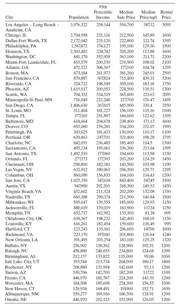
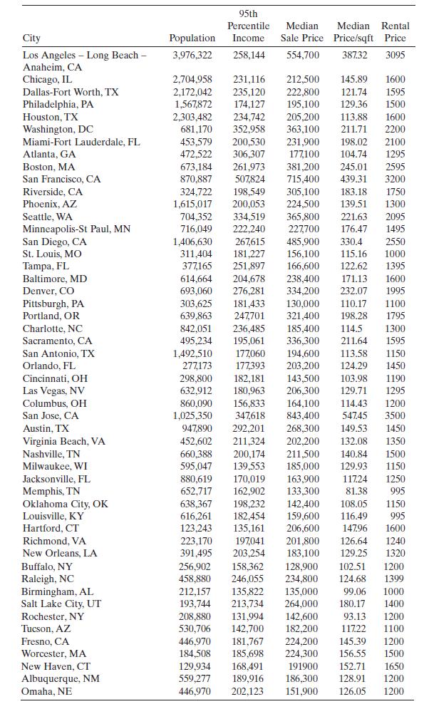
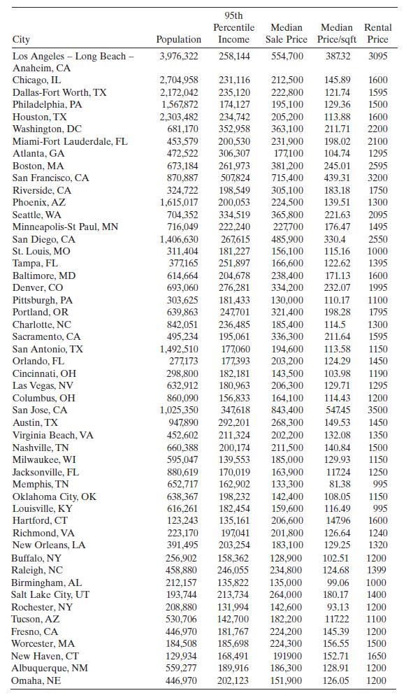
Table B. 24 contains data on home rental prices and home sales. Use all possible regressions to build a model for these data. Perform a residual analysis on the final model and comment on model adequacy. City 95th Percentile Median Median Rental Population Income Sale Price Price/sqft Price Los
Use stepwise regression to build a model for the home rental prices and home sales data in Table B.24. Perform a residual analysis on the final model. Compare this model to the all possible regressions model from Problem 10.40.Data From Problem 10.40Table B. 24 contains data on home rental prices
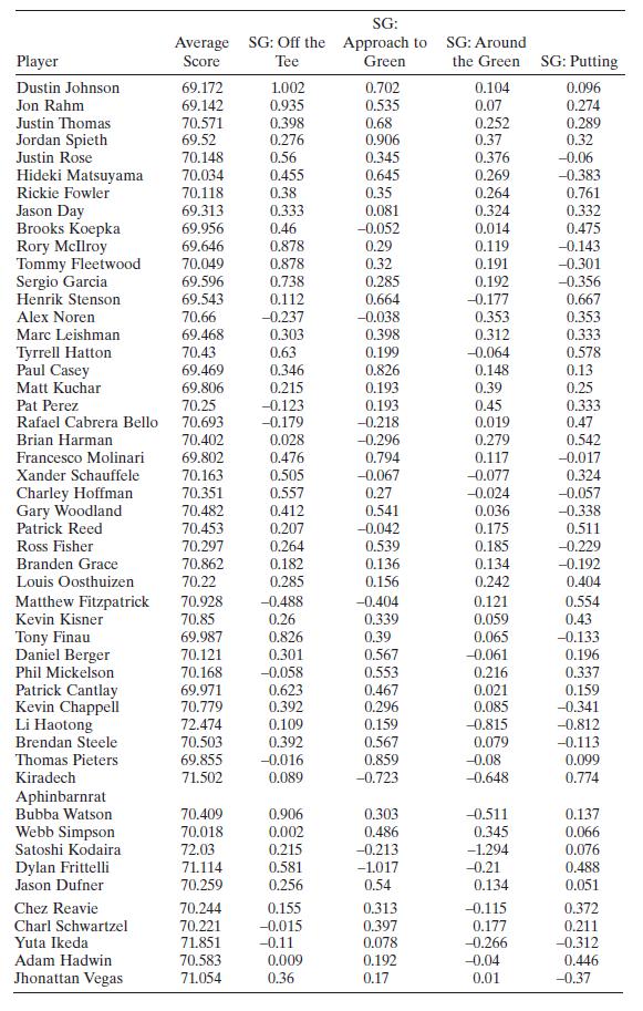
Table B. 25 contains the golf data on strokes gained. Use all possible regressions to build a model for these data. Perform a residual analysis on the final model and comment on model adequacy. SG: Average SG: Off the Approach to SG: Around Player Score Tee Green the Green SG: Putting Dustin
Consider the regression model developed for the National Football League data in Problem 3.1.Data From Problem 3.1Consider the National Football League data in Table B.1.a. Calculate the PRESS statistic for this model. What comments can you make about the likely predictive performance of this
Split the National Football League data used in Problem 3.1 into estimation and prediction data sets. Evaluate the statistical properties of these two data sets. Develop a model from the estimation data and evaluate its performance on the prediction data. Discuss the predictive performance of this
Calculate the PRESS statistic for the model developed from the estimation data in Problem 11.2. How well is the model likely to predict? Compare this indication of predictive performance with the actual performance observed in Problem 11.2.Data From Problem 11.2Split the National Football League
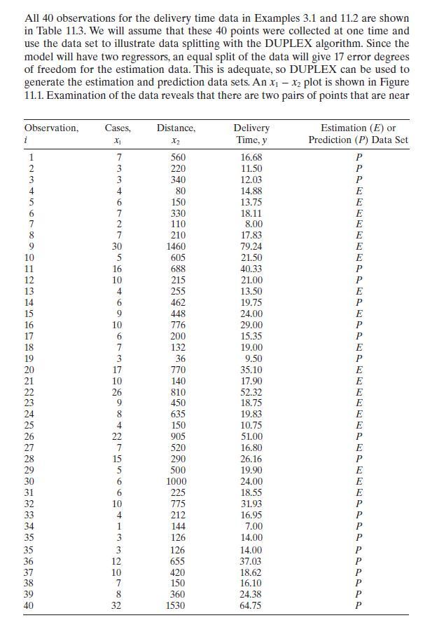
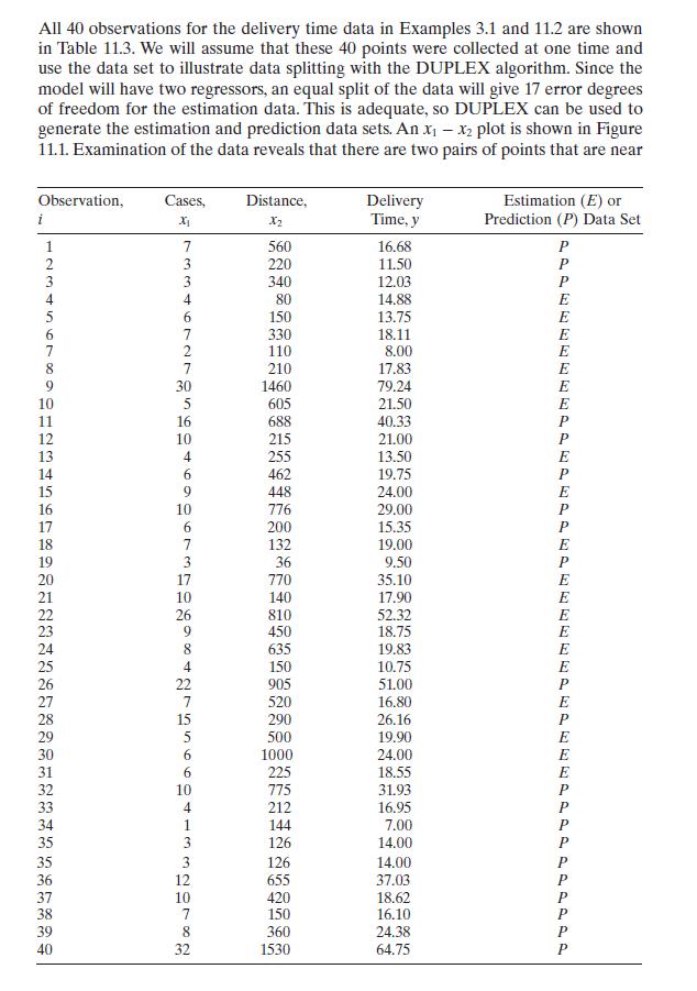
Consider the delivery time data discussed in Example 11.3. Find the PRESS statistic for the model developed from the estimation data. How well is the model likely to perform as a predictor? Compare this with the observed performance in prediction.Data From Example 11.3 i All 40 observations for the
Consider the delivery time data discussed in Example 11.3.Data From Example 11.3a. Develop a regression model using the prediction data set.b. How do the estimates of the parameters in this model compare with those from the model developed from the estimation data? What does this imply about model
In Problem 3.5 a regression model was developed for the gasoline mileage data using the regressor engine displacement \(x_{1}\) and number of carburetor barrels \(x_{6}\). Calculate the PRESS statistic for this model. What conclusions can you draw about the model's likely predictive
In Problem 3.6 a regression model was developed for the gasoline mileage data using the regressor vehicle length \(x_{8}\) and vehicle weight \(x_{10}\). Calculate the PRESS statistic for this model. What conclusions can you draw about the potential performance of this model as a predictor?Data
Consider the gasoline mileage data in Table B.3. Delete eight observations (chosen at random) from the data and develop an appropriate regression model. Use this model to predict the eight withheld observations. What assessment would you make of this model's predictive performance? Automobile y X2
Consider the gasoline mileage data in Table B.3. Split the data into estimation and prediction sets.a. Evaluate the statistical properties of these data sets.b. Fit a model involving \(x_{1}\) and \(x_{6}\) to the estimation data. Do the coefficients and fitted values from this model seem
Refer to Problem 11.2. What are the standard errors of the regression coefficients for the model developed from the estimation data? How do they compare with the standard errors for the model in Problem 3.5 developed using all the data?Data From Problem 11.2Split the National Football League data
Refer to Problem 11.2. Develop a model for the National Football League data using the prediction data set.Data From Problem 11.2Split the National Football League data used in Problem 3.1 into estimation and prediction data sets. Evaluate the statistical properties of these two data sets. Develop
What difficulties do you think would be encountered in developing a computer program to implement the DUPLEX algorithm? For example, how efficient is the procedure likely to be for large sample sizes? What modifications in the procedure would you suggest to overcome those difficulties?
If \(\mathbf{Z}\) is the \(n \times k\) matrix of standardized regressors and \(\mathbf{T}\) is the \(k \times k\) upper triangular matrix in Eq. (11.3), show that the transformed regressors \(\mathbf{W}=\mathbf{Z T}^{-1}\) are orthogonal and have unit variance.Equation 11.3 W = ZT-1
Show that the least-squares estimate of \(\boldsymbol{\beta}\) (say \(\hat{\boldsymbol{\beta}}_{(i)}\) ) with the \(i\) th observation deleted can be written in terms of the estimate based on all \(n\) points as\[\hat{\beta}_{(i)}=\hat{\beta}-\frac{e_{i}}{1-h_{i i}}\left(\mathbf{X}^{\prime}
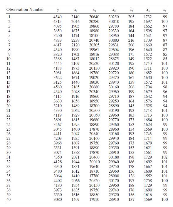
Consider the heat treating data in Table B.12. Split the data into prediction and estimation data sets.a. Fit a model to the estimation data set using all possible regressions. Select the minimum \(C_{p}\) model.b. Use the model in part a to predict the responses for each observation in the
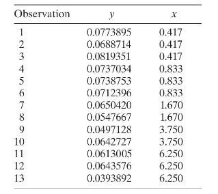
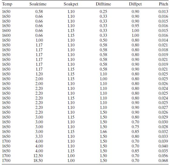
Consider the jet turbine engine thrust data in Table B.13. Split the data into prediction and estimation data sets.a. Fit a model to the estimation data using all possible regressions. Select the minimum \(C_{p}\) model.b. Use the model in part a to predict each observation in the prediction data
Consider the electronic inverter data in Table B.14. Delete the second observation in the data set. Split the remaining observations into prediction and estimation data sets.a. Find the minimum \(C_{p}\) equation for the estimation data set.b. Use the model in part a to predict each observation in
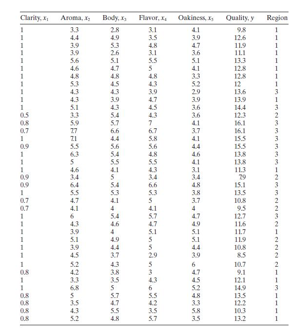
Table B. 11 presents 38 observations on wine quality.a. Select four observations at random from this data set, then delete these observations and fit a model involving only the regressor flavor and the indicator variables for the region information to the remaining observations. Use this model to
Consider all 40 observations on the delivery time data. Delete \(10 \%\) (4) of the observations at random. Fit a model to the remaining 36 observations, predict the four deleted values, and calculate \(R^{2}\) for prediction. Repeat these calculations 100 times. Calculate the average \(R^{2}\) for
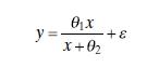
Consider the Michaelis-Menten model introduced in Eq. (12.23). Graph the expectation function for this model for \(\theta_{1}=200\) and \(\theta_{2}=0.04,0.06,0.08\), 0.10 . Overlay these curves on the same set of \(x-y\) axes. What effect does the parameter \(\theta_{2}\) have on the behavior of
Consider the Michaelis-Menten model introduced in Eq. (12.23). Graph the expectation function for \(\theta_{1}=100,150,200,250\) for \(\theta_{2}=0.06\). Overlay these curves on the same set of \(x-y\) axes. What effect does the parameter \(\theta_{1}\) have on the behavior of the expectation
Graph the expectation function for the logistic growth model (12.34) for \(\theta_{1}=10, \theta_{2}=2\), and values of \(\theta_{3}=0.25,1,2,3\), respectively. Overlay these plots on the same set of \(x-y\) axes. What effect does the parameter \(\theta_{3}\) have on the expectation
Consider the National Football League data in Table B.1.a. Use the forward selection algorithm to select a subset regression model.b. Use the backward elimination algorithm to select a subset regression model.c. Use stepwise regression to select a subset regression model.d. Comment on the final
Consider the National Football League data in Table B.1. Restricting your attention to regressors \(x_{1}\) (rushing yards), \(x_{2}\) (passing yards), \(x_{4}\) (field goal percentage), \(x_{7}\) (percent rushing), \(x_{8}\) (opponents' rushing yards), and \(x_{9}\) (opponents' passing yards),
In stepwise regression, we specify that \(F_{\mathrm{IN}} \geq F_{\mathrm{OUT}}\left(\right.\) or \(t_{\mathrm{IN}} \geq t_{\mathrm{OUT}}\) ). Justify this choice of cutoff values.
Consider the solar thermal energy test data in Table B.2.a. Use forward selection to specify a subset regression model.b. Use backward elimination to specify a subset regression model.c. Use stepwise regression to specify a subset regression model.d. Apply all possible regressions to the data.
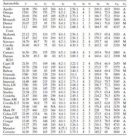
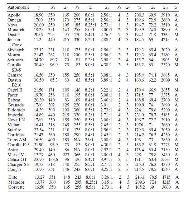
Consider the gasoline mileage performance data in Table B.3.a. Use the all-possible-regressions approach to find an appropriate regression model.b. Use stepwise regression to specify a subset regression model. Does this lead to the same model found in part a? Automobile X1 x2 X3 X4 Apollo 18.90 350
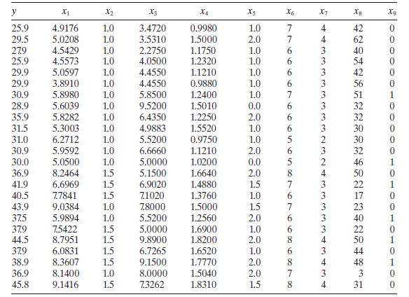
Consider the property valuation data found in Table B.4.a. Use the all-possible-regressions method to find the "best" set of regressors.b. Use stepwise regression to select a subset regression model. Does this model agree with the one found in part a? y X1 X2 X4 Xs X6 X7 5 X8 Xg 25.9 4.9176 1.0
Use stepwise regression with \(F_{\mathrm{IN}}=F_{\text {OUT }}=4.0\) to find the "best" set of regressor variables for the Belle Ayr liquefaction data in Table B.5. Repeat the analysis with \(F_{\mathrm{IN}}=F_{\mathrm{OUT}}=2.0\). Are there any substantial differences in the models obtained? Run
Use the all-possible-regressions method to select a subset regression model for the Belle Ayr liquefaction data in Table B.5. Evaluate the subset models using the \(C_{p}\) criterion. Justify your choice of final model using the standard checks for model adequacy. Run No. y X x2 X3 X4 Xs X6
Analyze the tube-flow reactor data in Table B. 6 using all possible regressions. Evaluate the subset models using the \(R_{p}^{2}, C_{p}\), and \(M S_{\text {Res }}\) criteria. Justify your choice of final model using the standard checks for model adequacy. Run No. y X X2 X4 11 28
Analyze the air pollution and mortality data in Table B. 15 using all possible regressions. Evaluate the subset models using the \(R_{p}^{2}, C_{p}\), and \(M S_{\text {Res }}\) criteria. Justify your choice of the final model using the standard checks for model adequacy.a. Use the
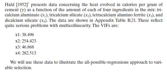
Consider the all-possible-regressions analysis of Hald's cement data in Example 10.1. If the objective is to develop a model to predict new observations, which equation would you recommend and why?Example 10.1 Hald [1952] presents data concerning the heat evolved in calories per gram of cement (y)
Consider the all-possible-regressions analysis of the National Football League data in Problem 10.2. Identify the subset regression models that are \(R^{2}\) adequate (0.05).Data From Problem 10.2Consider the National Football League data in Table B.1. Restricting your attention to regressors

Showing 1600 - 1700 of 2175

First
8
9
10
11
12
13
14
15
16
17
18
19
20
21
22

Step by Step Answers

Services

Sitemap
Fun
Definitions
Become Tutor
Used Textbooks
Study Help Categories
Recent Questions
Expert Questions
Campus Wear
Sell Your Books

Company Info

Security
Copyrights
Privacy Policy
Terms & Conditions
SolutionInn Fee
Scholarship
Online Quiz
Give Feedback, Get Rewards

Get In Touch

About Us
Contact Us
Career
Jobs
FAQ
Student Discount
Campus Ambassador

Secure Payment

Download Our App

© 2026 SolutionInn. All Rights Reserved