New Semester
Started
Get
50% OFF
Study Help!
--h --m --s
Claim Now
Question Answers
Textbooks
Find textbooks, questions and answers
Oops, something went wrong!
Change your search query and then try again
S
Books
FREE
Study Help
Expert Questions
Accounting
General Management
Mathematics
Finance
Organizational Behaviour
Law
Physics
Operating System
Management Leadership
Sociology
Programming
Marketing
Database
Computer Network
Economics
Textbooks Solutions
Accounting
Managerial Accounting
Management Leadership
Cost Accounting
Statistics
Business Law
Corporate Finance
Finance
Economics
Auditing
Tutors
Online Tutors
Find a Tutor
Hire a Tutor
Become a Tutor
AI Tutor
AI Study Planner
NEW
Sell Books
Search
Search
Sign In
Register
study help
computer science
systems analysis design
System Engineering Analysis Design And Development Concepts Principles And Practices Wiley Series In Systems Engineering And Management 2nd Edition Charles S. Wasson - Solutions
What is an architecture?
What is an AD?
What are the differences between User views, viewpoints, and concerns and provide examples?
What roles do the System Architect and SE perform regarding User views, viewpoints, and concerns?
What are the differences and interrelationships between architecting versus engineering versus designing?
Is System Architecting a 1-hour block diagram exercise?If not, explain why?
What is a fault-tolerant architecture and what is its purpose?
Who performs a System Architect role on small, medium, and large projects?
Pick one of the following Systems or Products listed below. Describe: 1) what information the Monitor capability provides as a Situational Assessment to the User and 2) what controls are available for the User to Command & Control (C2) it:a. Aircraftb. Automobilec. Desktop, laptop, or tablet
Identify three examples of each of the types of system architectures listed below:a. Centralized architectureb. Decentralized architecture
Identify an example of each of the types of redundancies listed below:a. Operational or Hot Standby redundancyb. Cold or standby redundancyc. “k-out-of-n” redundancy
Identify an example of each of the types of component implementation redundancies listed below:a. Like redundancyb. Unlike redundancyc. Data link redundancyd. Physical connectivity redundancy (Figure 26.12) Hydraulics 3 FWD Hydraulics 1 Fan Disk Hydraulics 2 Elevator Actuator (4 per airplane)
How are System interfaces identified?
How do SEs analyze interface interactions?
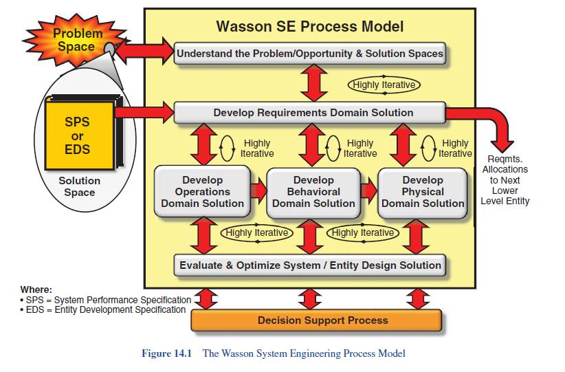
Howdoes the SE Process (Figure 14.1) apply to interface design? Problem Space Wasson SE Process Model Understand the Problem/Opportunity & Solution Spaces Highly Iterative SPS or EDS Develop Requirements Domain Solution Highly Iterative Highly Iterative 10 Highly Iterative Solution Space Develop
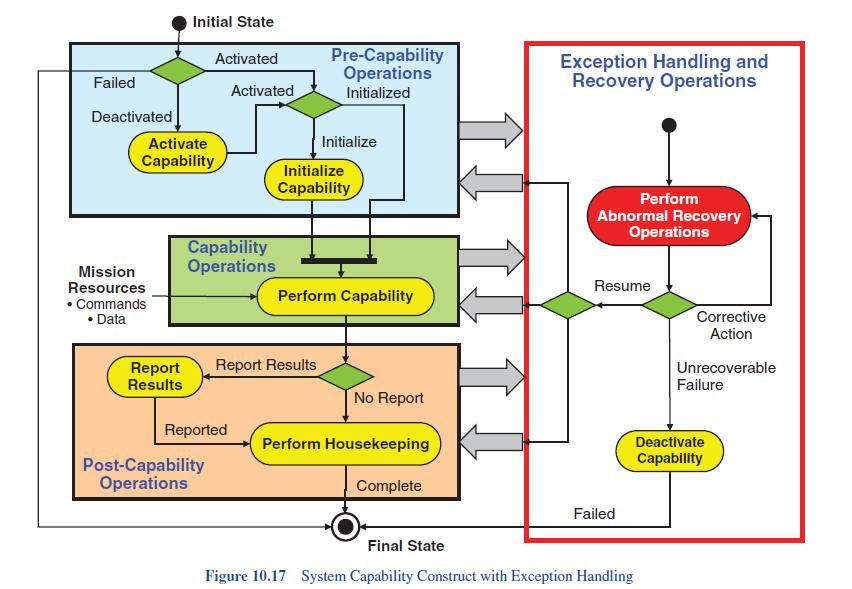
How does the System Capability Construct (Figure 10.17) apply to interface design? Failed Initial State Activated Activated Deactivated Activate Pre-Capability Operations Initialized Exception Handling and Recovery Operations Initialize Capability Initialize Capability Perform Abnormal Recovery
What is the methodology for defining interfaces?
Who owns and controls System or Entity interfaces at various levels of abstraction?
What is an IRS and what is its relationship to interface definition?
What is an ICD and what is its relationship to interface design?
What is an IDD and what is its relationship to interface design?
How to determine whether to develop an IRS, ICD, and/or IDD?
What is an ICWG and what is its relationship to a System Development project?
How is the membership composition of an ICWG determined technically?
Who chairs an ICWG?
What are some of the challenges of analyzing, designing, and controlling System or Entity interfaces?
Create your own definition of a system. Based on the“system” definitions provided in this chapter:a. Identify your viewpoint of shortcomings in the definitions.b. Provide rationale as to why you believe your definition overcomes those shortcomings.
From a historical perspective, identify three precedented systems that were replaced with unprecedented systems.
What is a system?
Is a product a system?
Is a service a system?
What are examples of different types of systems?
What are the two primary types of systems associated with system, product, or service development?
What is an Engineered System?
What is an Organizational System?
What is Engineering?
What is SE?
SE consists of three primary aspects. What are they?Describe the interactions among the three.
How does the scope of Engineering compare with SE in terms of “Engineering the System” versus “Engineering the Box.”
What is the difference between a system, a product, and a tool?
What is a paradigm?
What is meant by a paradigm shift?
What is verification?
What is validation?
What is the Plug and Chug … SDBTF paradigm? What are its origins? Why is it important to get the SDBTF Paradigm corrected in Engineering education?
What does “Paint by Number” Engineering refer to?What are its pros and cons?
What is Lean Thinking?
What is Lean SE?
What are Lean SE Principles intended to accomplish?
Why does application of Lean SE principles to an SDBTF-DPM Engineering Process result in another SDBTF-DPM Engineering Process
What is a SOI?
What is the difference between a capability and a function?
What is the top level system analytical construct?
What do systems interact with?
What is a system attribute?
What is a system property?
What is a system characteristic?
What makes a system, product, or service unique?
What influences a system and its results?
What are some types of system characteristics?
What constitutes a system’s state of equilibrium and stability?
What is a system life cycle?
From an SE perspective, what criteria should a life cycle meet?
What is the System Definition Phase, when does it start, and when does it end?
What is the System Procurement Phase, when does it start, and when does it end?
What is the System Development Phase, when does it start, and when does it end?
What is the System Production Phase, when does it start, and when does it end?
What is the System Operations, Maintenance, and Support (OM&S) Phase, when does it start, and when does it end?
What is the System Retirement and Disposal Phase, when does it start, and when does it end?
What is a Mission System (Producer) role?
What is an Enabling System (Supplier) role?
What is a Problem Space?
What is an Opportunity Space?
What is the relationship between a Problem Space and an Opportunity Space?
What is a Solution Space?
What is the relationship between the Problem/Opportunity Space and a Solution Space?
How do you write a Problem Statement?
Identify three rules for writing Problem Statements.
How do you forecast the Problem Spaces?
How does an Enterprise resolve gaps between a Problem Space and its Solution Space(s)?
Where and how do Users obtain system requirements for development?
Cite various Solution Space tools that enable a homeowner to leverage their time, resources, and skills to maintain their lawn.
Cite two examples of Human Systems—organizational and engineered—that project or expand their sphere of influence by leveraging the capabilities of other systems.
How does System Definition vary between consumer product development and contract system development?
What is a mission?
Is the term “mission” restricted to the military applications?Explain why?
Do consumer products and services perform missions?
How do you plan a mission?
What is a Mission Event Timeline (MET), its key attributes, and how is it developed.
How is mission task analysis is performed?
What are the primary phases of operation of a system, product, or service? Can there be other phases of operation?
What system operations and decisions are performed during the Pre-Mission, Mission, and Post-Mission Phases?
How do SEs bound each mission phase of operation and establish criteria for triggering the next phase? Why is it important to bound phases of operation? What occurs if you do not bound each phase of operation?
What is a User Story?
How many UCs does a system, product, or service need?
Which types of systems employ UCs? Organizations, systems, products, or services; Subsystems, or Assemblies?
What are the attributes of a UC?
What is UC analysis and how do you perform one?
What is an Actor and what is its relationship to a UC?
Is each UC restricted to one Actor?
Showing 1800 - 1900
of 5433
First
12
13
14
15
16
17
18
19
20
21
22
23
24
25
26
Last
Step by Step Answers