Consider the satellite described in Problem 11.4-8. The plant model is given as

The plant disturbances are caused by random variations in the Earth’s gravity field. Suppose that R_w = 1 and R_v = 0.02.

(a) The measurement y(k) is in the units of angular degrees and is obtained from a stable platform. Describe the accuracy of this measurement; that is, what does the value of Rv tell us about the sensor accuracy?

(b) Calculate and plot the Kalman gains, as in Fig. 11-5, using M(0) = I .

(c) The diagonal elements of the steady-state error covariance matrix are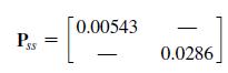

Comment on the steady-state accuracy of this Kalman filter.

(d) The LQ design of Problem 11.4-8 yielded the steady-state gains of K = [0.51922.103]. Find the transfer function Dce(z) of the control estimator.

(e) Calculate and plot the Nyquist diagram for the closed-loop system opened at the plant input. What are the phase and gain margins?

Problem 11.4-8

Consider the third-order continuous-time LTI system

Fig. 11-5

Transcribed Image Text:

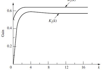
= [1 ]x) + x(k) y(k)= [10]x(k) + (k) x(k + 1) [0.11 Ju(k) + [0.02] 0.2 w(k)