Consider the simple treatment effect model \(y_{i}=\beta_{1}+\beta_{2} d_{i}+e_{i}\). Suppose that \(d_{i}=1\) or \(d_{i}=0\) indicating that a treatment is given to randomly selected individuals or not. The dependent variable \(y_{i}\) is the outcome variable. See the discussion of the difference estimator in Section 7.5.1. Suppose that \(N_{1}\) individuals are given the treatment and \(N_{0}\) individual are in the control group, who are not given the treatment. Let \(N=N_{0}+N_{1}\) be the total number of observations.

a. Show that if \(\operatorname{var}\left(e_{i} \mid \mathbf{d}\right)=\sigma^{2}\) then the variance of the OLS estimator \(b_{2}\) of \(\beta_{2}\) is \(\operatorname{var}\left(b_{2} \mid \mathbf{d}\right)=N \sigma^{2} /\left(N_{0} N_{1}\right)\). [Hint: See Appendix 7B.]

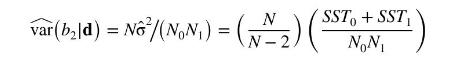
b. Let \(\bar{y}_{0}=\sum_{i=1}^{N_{0}} y_{i} / N_{0}\) be the sample mean of the outcomes for the \(N_{0}\) observations on the control group. Let \(S S T_{0}=\sum_{i=1}^{N_{0}}\left(y_{i}-\bar{y}_{0}\right)^{2}\) be the sum of squares about the sample mean of the control group, where \(d_{i}=0\). Similarly, let \(\bar{y}_{1}=\sum_{i=1}^{N_{1}} y_{i} / N_{1}\) be the sample mean of the outcomes for the \(N_{1}\) observations on the treated group, where \(d_{i}=1\). Let \(S S T_{1}=\sum_{i=1}^{N_{1}}\left(y_{i}-\bar{y}_{1}\right)^{2}\) be the sum of squares about the sample mean of the treatment group. Show that \(\hat{\sigma}^{2}=\sum_{i=1}^{N} \hat{e}_{i}^{2} /(N-2)=\left(S S T_{0}+S S T_{1}\right) /(N-2)\) and therefore that

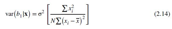
c. Using equation (2.14) find \(\operatorname{var}\left(b_{1} \mid \mathbf{d}\right)\), where \(b_{1}\) is the OLS estimator of the intercept parameter \(\beta_{1}\). What is \(\widehat{\operatorname{var}}\left(b_{1} \mid \mathbf{d}\right)\) ?

d. Suppose that the treatment and control groups have not only potentially different means but potentially different variances, so that \(\operatorname{var}\left(e_{i} \mid d_{i}=1\right)=\sigma_{1}^{2}\) and \(\operatorname{var}\left(e_{i} \mid d_{i}=0\right)=\sigma_{0}^{2}\). Find \(\operatorname{var}\left(b_{2} \mid \mathbf{d}\right)\). What is the unbiased estimator for \(\operatorname{var}\left(b_{2} \mid \mathbf{d}\right)\) ?

e. Show that the White heteroskedasticity robust estimator in equation (8.9) reduces in this case to \(\widehat{\operatorname{var}}\left(b_{2} \mid \mathbf{d}\right)=\frac{N}{N-2}\left(\frac{S S T_{0}}{N_{0}^{2}}+\frac{S S T_{1}}{N_{1}^{2}}\right)\). Compare this estimator to the unbiased estimator in part (d).

f. What does the robust estimator become if we drop the degrees of freedom correction \(N /(N-2)\) in the estimator proposed in part (e)? Compare this estimator to the unbiased estimator in part (d).

Data From Equation 2.14:-

Data From Equation 8.9:-

Transcribed Image Text:

= N SST+SST var (bld) = N /(NN) = (~~~2) (SS, + SST, N-2. NON