Consider the wage equation

where wage is measured in dollars per hour, education and experience are in years, and METRO \(=1\) if the person lives in a metropolitan area. We have \(N=1000\) observations from 2013.

a. We are curious whether holding education, experience, and METRO constant, there is the same amount of random variation in wages for males and females. Suppose \(\operatorname{var}\left(e_{i} \mid \mathbf{x}_{i}, F E M A L E=0\right)=\) \(\sigma_{M}^{2}\) and \(\operatorname{var}\left(e_{i} \mid \mathbf{x}_{i}, F E M A L E=1\right)=\sigma_{F}^{2}\). We specifically wish to test the null hypothesis \(\sigma_{M}^{2}=\sigma_{F}^{2}\) against \(\sigma_{M}^{2} eq \sigma_{F}^{2}\). Using 577 observations on males, we obtain the sum of squared OLS residuals, \(S S E_{M}=97161.9174\). The regression using data on females yields \(\hat{\sigma}_{F}=12.024\). Test the null hypothesis at the \(5 \%\) level of significance. Clearly state the value of the test statistic and the rejection region, along with your conclusion.

b. We hypothesize that married individuals, relying on spousal support, can seek wider employment types and hence holding all else equal should have more variable wages. Suppose \(\operatorname{var}\left(e_{i} \mid \mathbf{x}_{i}\right.\), MARRIED \(\left.=0\right)=\sigma_{\text {SINGLE }}^{2}\) and \(\operatorname{var}\left(e_{i} \mid \mathbf{x}_{i}\right.\), MARRIED \(\left.=1\right)=\sigma_{\text {MARRIED }}^{2}\). Specify the null hypothesis \(\sigma_{\text {SINGLE }}^{2}=\sigma_{\text {MARRIED }}^{2}\) versus the alternative hypothesis \(\sigma_{\text {MARRIED }}^{2}>\sigma_{\text {SINGLE }}^{2}\). We add FEMALE to the wage equation as an explanatory variable, so that

Using \(N=400\) observations on single individuals, OLS estimation of (XR8.6b) yields a sum of squared residuals is 56231.0382 . For the 600 married individuals, the sum of squared errors is \(100,703.0471\). Test the null hypothesis at the \(5 \%\) level of significance. Clearly state the value of the test statistic and the rejection region, along with your conclusion.

c. Following the regression in part (b), we carry out the \(N R^{2}\) test using the right-hand-side variables in (XR8.6b) as candidates related to the heteroskedasticity. The value of this statistic is 59.03. What do we conclude about heteroskedasticity, at the \(5 \%\) level? Does this provide evidence about the issue discussed in part (b), whether the error variation is different for married and unmarried individuals? Explain.

d. Following the regression in part (b) we carry out the White test for heteroskedasticity. The value of the test statistic is 78.82. What are the degrees of freedom of the test statistic? What is the 5\% critical value for the test? What do you conclude?

e. The OLS fitted model from part (b), with usual and robust standard errors, is

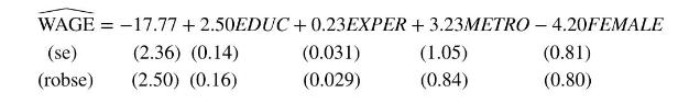
For which coefficients have interval estimates gotten narrower? For which coefficients have interval estimates gotten wider? Is there an inconsistency in the results?

f. If we add MARRIED to the model in part (b), we find that its \(t\)-value using a White heteroskedasticity robust standard error is about 1.0. Does this conflict with, or is it compatible with, the result in (b) concerning heteroskedasticity? Explain.

Transcribed Image Text:

WAGE; B+BEDUC; +3EXPER; + B4METRO + e (XR8.6a)